Getting started with python and influxdb

Alerting the DevOps Team on Service Failure

Visualizing service failure is great but you don’t want to be staring at Grafana every second and wait for a service failure.

Ideally, you would want to be notified via Slack for example in order to take immediate action over the failure.

This is exactly what we are going to configure on Grafana: Slack alerts.

In Grafana, you’ll be able to create some alerts only for the graph panel. Two steps and we are done.

A: Creating a Notification Channel

Before creating the actual alert, we have to create a notification channel. In the left menu, head over to the little bell icon, and click on “Notification Channels.”

When you’re there, you are presented with a couple of fields that you have to fill. As an example, I’ll give you my own configuration.

B: Creating the Alert

Now that our notification channel is created, it is time to build our final alert on the graph panel.

Head over to your dashboard, edit one of the graph panels and click on the little bell similar to the one on the left menu.

Again, I’ll provide a comprehensive screenshot on how I built my alerts.

This alert states that it will evaluate the last value provided by the query that you defined earlier for the last minute.

If it has no value, then an alert will be raised. The alert evaluation is done every 10 seconds.

You can reduce the “For” parameter too to 10s for your alert to be more reactive.

C: Emulating a Service Shutdown

Let’s pretend for a second that your Telegraf service is shutting down for no reason (it never happens in real life, of course.)

net stop telegraf

1	net stop telegraf

Here’s the graphical result in Grafana, along with the alert raised in Slack:

Done! We finally got what the reward of this hard work. Congratulations!

Quick Start for InfluxDB OSS

Select Quick Start in the last step of the InfluxDB user interface’s (UI)
to quickly start collecting data with InfluxDB.
Quick Start creates a data scraper that collects metrics from the InfluxDB endpoint.
The scraped data provides a robust dataset of internal InfluxDB metrics that you can query, visualize, and process.

Use Quick Start to collect InfluxDB metrics

After ,
the “Let’s start collecting data!” page displays options for collecting data.
Click Quick Start.

InfluxDB creates and configures a new scraper.
The target URL points to the HTTP endpoint of your local InfluxDB instance
(for example, ), which outputs internal InfluxDB
metrics in the Prometheus data format.
The scraper stores the scraped metrics in the bucket created during the
.

Quick Start is only available in the last step of the setup process.
If you missed the Quick Start option, you can manually create a scraper
that scrapes data from the endpoint.

Installing the Different Tools

Now that we know exactly what we are going to build, let’s install the different tools that we need.

A: Installing InfluxDB

Before configuring any monitoring agent, it is important to have a time series database first.

Launching Telegraf without InfluxDB would result in many error messages that won’t be very relevant.

Installing InfluxDB is pretty straightforward, head over to the download page and save the resulting .zip somewhere on your computer.

When saved, unzip the content wherever you want, launch a command line and navigate to the folder where you stored your binaries (in my case, directly in Program Files). Once there, you will be presented with a couple of files:

• exe: an CLI executable used to navigate in your databases and measurements easily;
• exe: used to launch an InfluxDB instance on your computer;
• exe: an executable used to run stress tests on your computer;
• influx_inspect: used to inspect InfluxDB disks and shards (not relevant in our case).

In our case, you want to run the influxd executable. Immediately after, you should see your InfluxDB instance running.

Launching InfluxDB On Windows.

InfluxDB does not ship as a service yet, even if it is completely doable to configure it as a user-defined service on Windows.

B: Installing Telegraf

Telegraf installation on Windows can be a bit tricky.

To download Telegraf, head over the InfluxDB downloads page and click on the latest version of Telegraf available.

Telegraf installation should be done in the Program Files folder, in a folder named Telegraf.

Launch a Powershell instance as an administrator. Head over to the Program Files folder and run:

mkdir Telegraf

1	mkdir Telegraf

Drop the executables downloaded here, and run:

telegraf.exe –service install

1	telegraf.exe–service install

As a consequence, Telegraf should be installed as a service and available in Windows services. Telegraf configuration file should be configured to retrieve metrics from your CPU and disk. To test it, run:

net start telegraf

1	net start telegraf

To check it, head over to InfluxDB folder (where you dropped your executables) and run influx.exe.If everything is running okay, you should start seeing metrics aggregating in InfluxDB.

You should be presented with a CLI, where you’ll type your first IFQL queries.

> show databases;
# You should see a list of your databases, including telegraf> use telegraf;
# Navigating in your telegraf database> show measurements;
# Getting the list of your measurements> SELECT * FROM win_cpu
# Seeing your CPU metrics

1 2 3 4 5

>show databases; # You should see a list of your databases, including telegraf> use telegraf; # Navigating in your telegraf database> show measurements; # Getting the list of your measurements> SELECT * FROM win_cpu # Seeing your CPU metrics

If you are unfamiliar with basics of InfluxDB and what IFQL is, check my ultimate InfluxDB guide for beginners. It contains good explanations regarding everything that you need to know.

C: Installing Grafana

For this tutorial, we are going to use the brand new Grafana v6.

Head over to Grafana download page, download the zip and unzip it wherever you want. Similarly to what you did with InfluxDB, head over to the folder where you stored your executables and run the Grafana server (grafana-server.exe in bin folder).

By default, Grafana will run on port 3000. Default credentials are admin/admin (you are prompted to modify them directly at boot time).

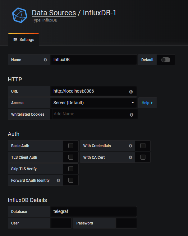
When you’re done, you’ll be asked to configure your data sources. By default, an InfluxDB instance runs on port 8086. The following configuration should do the trick:

Now that all the tools are configured, it is time to start monitoring Windows services.

Building an awesome dashboard

This is where the fun begins.

We are going to build our dashboard in Grafana v6.0.

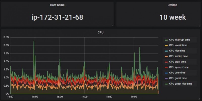
As a reminder, this is the dashboard that we are going to build today.

In Grafana, create a new dashboard by clicking on the plus icon on the left menu.

We chose the “Elapsed Time” metric in order to measure if services are up or down.

However, we have to perform transformations on our data as the Elapsed Time function is theoretically a never-ending growing function.

As I already did it in my article on systemd services, I will give you the widget and the query for you to reproduce this dashboard.

a – Building the performance gauge

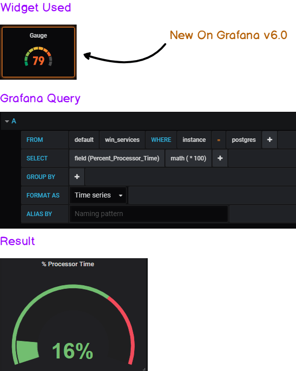
If you want to exact same output for the gauge, head over to the Visualization Panel: in the “Value Panel,” show the ‘Last’ value and select a “percent” unit.

b – Building the “availability” graph

The key here is the difference operator.

It gives the graph a “heartbeat” look that avoids having a growing graph that rescales permanently.

If you want to have the exact same output, head over to the “Visualization” panel and click on the “Staircase” option.

The other boxes of this dashboard are just plain text panels with some CSS color, nothing special here.

You can of course tweak the examples to monitor the services you are interested in and/or modify the query to take an operator that you find more suitable to your needs.

Now that our visualization is ready, it is time to warn our DevOps team every time a service fails.

Configuring Telegraf

Before creating our awesome dashboard, we need to configure Telegraf in order for it to query the Performance Counters API we described in the first chapter.

This will be done by using the win_perf_counters plugin of Telegraf. The plugin needs to be declared in the inputs section of your configuration file. It looks like this:

]
]
# Processor usage, alternative to native, reports on a per core.
ObjectName = “Processor”
Instances =
Counters =
Measurement = “win_cpu”

1 2 3 4 5 6 7

inputs.win_perf_counters inputs.win_perf_counters.object # Processor usage, alternative to native, reports on a per core. ObjectName=“Processor” Instances=“*” Counters=“%Idle Time”,“%Interrupt Time”,“%Privileged Time”,“%User Time” Measurement=“win_cpu”

The ObjectName property expects the exact same name that you would find the Performance Monitor. When in doubt about what you can query on Windows, you can either:

In our case, we want to monitor the Process object name, the ElapsedTime counter for the service we are interested in : postgres (for this example).

We can also add the % Processor Time metric in order to stop CPU-consuming resources.

The resulting Telegraf configuration will be:

]
]
# Processor usage, alternative to native, reports on a per core.
ObjectName = “Process”
Instances =
Counters =
Measurement = “win_services”

1 2 3 4 5 6 7

inputs.win_perf_counters inputs.win_perf_counters.object # Processor usage, alternative to native, reports on a per core. ObjectName=“Process” Instances=“*” Counters=“Elapsed Time”,“%Processor Time” Measurement=“win_services”

Now that everything is configured, let’s head over to Grafana and build our dashboard.

5: Установка и настройка Chronograf

Chronograf – это приложение визуализации данных, которое позволяет строить графики на основе отслеженных данных и создавать правила оповещения и автоматизации. Chronograf поддерживает шаблоны и предоставляет библиотеку предварительно настроенных удобных дашбордов для общих наборов данных. Установите Chronograf и подключите его к другим компонентам стека.

Загрузите и установите последнюю версию:

Запустите сервис Chronograf:

Примечание: Если вы включили брандмауэр ufw, разблокируйте порт 8888:

Откройте в браузере интерфейс Chronograf:

Вы увидите приветственную страницу приложения:

Введите имя и пароль пользователя InfluxDB, а затем нажмите Connect New Source.

После этого вы увидите список хостов. Кликните на имя хоста вашего сервера, чтобы открыть дашборд и просмотреть ряд графиков системного уровня.

Теперь нужно подключить Chronograf к Kapacitor для отправления оповещений.

Наведите курсор на последний элемент в левом меню навигации и нажмите Kapacitor, чтобы открыть страницу конфигурации.

Используйте данные подключения по умолчанию (в руководстве имя пользователя и пароль для Kapacitor не были установлены). Нажмите Connect Kapacitor. Как только Kapacitor успешно подключится, вы увидите раздел Configure Alert Endpoints.

Kapacitor поддерживает несколько конечных точек для отправки оповещений:

• HipChat
• OpsGenie
• PagerDuty
• Sensu
• Slack
• SMTP
• Talk
• Telegram
• VictorOps

InfluxDB Clustering

I last blogged about InfluxDB clustering a while ago and thought it was time to update you with a feature that is only available in our commercial product offerings — InfluxDB Cloud and InfluxDB Enterprise.

Architectural Overview

InfluxDB Clustering Overview

An InfluxDB Enterprise installation allows for a clustered InfluxDB installation which consists of two separate software processes: Data nodes and Meta nodes. To run an InfluxDB cluster, both the meta and data nodes are required.

The meta nodes expose an HTTP API that the command uses. This command is what system operators use to perform operations on the cluster like adding and removing servers, moving shards (large blocks of data) around a cluster and other administrative tasks. They communicate with each other through a TCP Protobuf protocol and a Raft consensus group.

Data nodes communicate with each other through a TCP and Protobuf protocol. Within a cluster, all meta nodes must communicate with all other meta nodes. All data nodes must communicate with all other data nodes and all meta nodes.

The meta nodes keep a consistent view of the metadata that describes the cluster. The meta-cluster uses the HashiCorp implementation of Raft as the underlying consensus protocol. This is the same implementation that they use in Consul. The meta nodes can run on very modestly sized VMs (t2-micro is sufficient in most cases).

The data nodes replicate data and query each other via a Protobuf protocol over TCP. Details on replication and querying are covered in the documentation. Data nodes are responsible for handling all writes and queries. Sizing is dependent on your schema and your write and query load.

Optimal Server Counts

For optimal InfluxDB Clustering, you’ll need to choose how many meta and data nodes to configure and connect. You can think of InfluxDB Enterprise as two separate clusters that communicate with each other: a cluster of meta nodes and one of data nodes.

Meta Nodes: The magic number is 3!

The number of meta nodes is driven by the number of meta node failures they need to be able to handle, while the number of data nodes scales based on your storage and query needs.

The consensus protocol requires a quorum to perform any operation, so there should always be an odd number of meta nodes. For almost all use cases, 3 meta nodes is the correct number, and such a cluster will operate normally even with the loss of 1 meta node. A cluster with 4 meta nodes can still only survive the loss of 1 node. Losing a second node means the remaining two nodes can only gather two votes out of a possible four, which does not achieve a majority consensus. Since a cluster of 3 meta nodes can also survive the loss of a single meta node, adding the fourth node achieves no extra redundancy and only complicates cluster maintenance. At higher numbers of meta nodes the communication overhead increases exponentially, so a configuration of 5 meta nodes is likely the max you’d ever want to have.

Data Nodes: Based on scalability requirements

Data nodes hold the actual time series data. The minimum number of data nodes to run is 1 and can scale up from there. Generally, you’ll want to run a number of data nodes that is evenly divisible by your replication factor. For instance, if you have a replication factor of 2, you’ll want to run 2, 4, 6, 8, 10, etc. data nodes. However, that’s not a hard and fast rule, particularly because you can have different replication factors in different retention policies.

InfluxDB Clustering and Where Data Lives

The meta and data nodes are each responsible for different parts of the database.

Meta Nodes: Meta nodes hold all of the following meta data:

• all nodes in the cluster and their role
• all databases and retention policies that exist in the cluster
• all shards and shard groups, and on what nodes they exist
• cluster users and their permissions
• all continuous queries

Data Notes: Data nodes hold all of the raw time series data and metadata, including:

• measurements
• tag keys and values
• field keys and values

• I would recommend you try out our InfluxDB clustering solution by either starting a InfluxDB Cloud or InfluxDB Enterprise Trial.
• Read the documentation on Clustering
• Learn about the features and usage of InfluxDB Cloud and InfluxDB Enterprise.

Step 2 – Configuring Telegraf

Telegraf provides a command for generating a sample config that includes all plugins and outputs:, but for the purposes of this guide, we will use a more simple config file, paste the configuration found below into a file called . You will need to edit the two indicated lines to match your environment if necessary.

    dc = "us-east-1"

# OUTPUTS


    # The full HTTP endpoint URL for your InfluxDB instance
    url = "http://localhost:8086" # EDIT THIS LINE
    # The target database for metrics. This database must already exist
    database = "telegraf" # required.


    # URLs of kafka brokers
    brokers =  # EDIT THIS LINE
    # Kafka topic for producer messages
    topic = "telegraf"

# PLUGINS
# Read metrics about cpu usage

    # Whether to report per-cpu stats or not
    percpu = false
    # Whether to report total system cpu stats or not
    totalcpu = true

Installing the different tools

Now that we know exactly what we are going to build, let’s install the different tools that we need.

a – Installing InfluxDB

Before configuring any monitoring agent, it is important to have a time series database first.

Launching Telegraf without InfluxDB would result in many error messages that won’t be very relevant.

Installing InfluxDB is pretty straightforward, head over to https://portal.influxdata.com/downloads/ and save the resulting .zip somewhere on your computer.

When saved, unzip the content wherever you want, launch a command line and navigate to the folder where you stored your binaries (in my case, directly in Program Files). Once there, you will be presented with a couple of files:

• influx.exe: an CLI executable used to navigate in your databases and measurements easily;
• influxd.exe: used to launch an InfluxDB instance on your computer;
• influx_stress.exe: an executable used to run stress tests on your computer;
• influx_inspect: used to inspect InfluxDB disks and shards (not relevant in our case).
• In our case, you want to run the influxd executable. Immediately after, you should see your InfluxDB instance running.

InfluxDB does not ship as a service yet, even if it is completely doable to configure it as a user-defined service on Windows.

b – Installing Telegraf

Telegraf installation on Windows can be a bit tricky.

To download Telegraf, head over to the InfluxDB downloads page and click on the latest version of Telegraf available.

Telegraf installation should be done in the Program Files folder, in a folder named Telegraf.

Launch a Powershell instance as an administrator. Head over to the Program Files folder and run:

Drop the executables downloaded here, and run:

As a consequence, Telegraf should be installed as a service and available in Windows services. Telegraf configuration file should be configured to retrieve metrics from your CPU and disk. To test it, run:

If everything is running okay, you should start seeing metrics aggregating in InfluxDB.

To check it, head over to InfluxDB folder (where you dropped your executables) and run influx.exe.

You should be presented with a CLI, where you’ll type your first IFQL queries.

If you are unfamiliar with basics of InfluxDB and what IFQL is, check my ultimate InfluxDB guide for beginners. It contains good explanations regarding everything that you need to know: https://devconnected.com/the-definitive-guide-to-influxdb-in-2019/

c – Installing Grafana

For this tutorial, we are going to use the brand new Grafana v6.

Head over to Grafana download page, download the zip and unzip it wherever you want. Similarly to what you did with InfluxDB, head over to the folder where you stored your executables and run the Grafana server (grafana-server.exe in bin folder).

By default, Grafana will run on port 3000. Default credentials are admin/admin (you are prompted to modify them directly at boot time).

When you’re done, you’ll be asked to configure your data sources. By default, an InfluxDB instance runs on port 8086. The following configuration should do the trick:

Now that all the tools are configured, it is time to start monitoring Windows services.

InfluxDB Python Client Library

While the influxdb-python library is hosted by InfluxDB’s GitHub account, it’s maintained by a trio of community volunteers, @aviau, @xginn8, and @sebito91. Many thanks to them for their hard work and contributions back to the community.

Installing the Library

Like many Python libraries, the easiest way to get up and running is to install the library using .

You should see some output indicating success.

No errors—looks like we’re ready to go!

Making a Connection

There are some additional parameters available to the  constructor, including username and password, which database to connect to, whether or not to use SSL, timeout and UDP parameters.

If you wanted to connect to a remote host at  on port  with username  and password  and using SSL, you could use the following command instead, which enables SSL and SSL verification with two additional arguments, and :

Now, let’s create a new database called  to store our data:

We can check if the database is there by using the  function of the client:

There it is, in addition to the  and  databases I have on my install. Finally, we’ll set the client to use this database:

Inserting Data

The  method has an argument called , which is a list of dictionaries, and contains the points to be written to the database. Let’s create some sample data now and insert it. First, let’s add three points in JSON format to a variable called :

These indicate “brush events” for our smart toothbrush; each one happens around 8AM in the morning, is tagged with the username of the person using the toothbrush and an ID of the brush itself (so we can track how long each brush head has been used for), and has a field which contains how long the user brushed for, in seconds.

Since we already have our database set, and the default input for  is JSON, we can invoke that method using our  variable as the only argument, as follows:

You should see the response  being returned by the function if the write operation has been successful. If you’re building an application, you’d want this collection of data to be automatic, adding points to the database every time a user interacts with the toothbrush.

Querying Data

In most cases you won’t need to access the JSON directly, however. Instead, you can use the  method of the  to get the measurements from the request, filtering by tag or field. If you wanted to iterate through all of Carol’s brushing sessions; you could get all the points that are grouped under the tag “user” with the value “Carol”, using this command:

 in this case is a Python Generator, which is a function that works similarly to an Iterator; you can iterate over it using a  loop, as follows:

Depending on your application, you might iterate through these points to compute the average brushing time for your user, or just to verify that there have been X number of brushing events per day.

If you were interested in tracking the amount of time an individual brush head has been used, you could substitute a new query that groups points based on the , then take the duration of each of those points and add it to a sum. At a certain point you could alert your user that it’s time to replace their brush head:

6: Создание оповещений

Наведите курсор на левое меню навигации, найдите раздел ALERTING и нажмите Kapacitor Rules. Затем нажмите Create New Rule.

В первом разделе выберите временной ряд, нажав на telegraf.autogen. Затем выберите систему из появившегося списка. После этого выберите load1. Вы сразу увидите соответствующий график в следующем разделе.

Над графиком найдите поле Send Alert where load1 is Greater Than и введите 1.0.

В поле Alert Message вставьте следующий текст:

Наведите кусор на записи в разделе Templates, чтобы получить описание каждого поля.

В выпадающем списке Send this Alert to выберите Smtp. Укажите почтовый адрес.

По умолчанию сообщения приходят в формате JSON.

Вы можете переименовать это правило. Для этого щелкните по его имени в верхнем левом углу страницы и введите новое имя.

Нажмите Save Rule в правом верхнем углу, чтобы завершить настройку этого правила.

Чтобы протестировать новое оповещение, создайте скачок CPU. Для этого используйте команду dd, которая будет читать данные из /dev/zero и отправлять их в /dev/null.

Пусть команда поработает несколько минут. Это создаст скачок CPU. Чтобы остановить команду, нажмите CTRL+C.

Через некоторое время вы получите сообщение на электронную почтуЧтобы просмотреть все предупреждения, нажмите Alert history в левом меню навигации пользовательского интерфейса Chronograf.

Примечание: Убедившись, что можете получать уведомления, не забудьте остановить команду dd. Просто нажмите CTRL+C.

Building an Awesome Dashboard

This is where the fun begins.

We are going to build our dashboard in Grafana v6.0.

As a reminder, this is the dashboard that we are going to build today.

In Grafana, create a new dashboard by clicking on the plus icon on the left menu.

We chose the “Elapsed Time” metric in order to measure if services are up or down.

However, we have to perform transformations on our data as the Elapsed Time function is theoretically a never-ending growing function.

As I already did it in my article on systemd services, I will give you the widget and the query for you to reproduce this dashboard.

A: Building the Performance Gauge

If you want to exact same output for the gauge, head over to the Visualization Panel: in the “Value Panel,” show the “Last” value and select a “percent” unit.

B: Building the ‘Availability’ Graph

The key here is the difference operator.

It gives the graph a “heartbeat” look that avoids having a growing graph that rescales permanently.

If you want to have the exact same output, head over to the “Visualization” panel and click on the “Staircase” option.

The other boxes of this dashboard are just plain text panels with some CSS color, nothing special here.

You can, of course, tweak the examples to monitor the services you are interested in and/or modify the query to take an operator that you find more suitable to your needs.

Now that our visualization is ready, it is time to warn our DevOps team every time a service fails.

Create a Telegraf configuration

1. Open the InfluxDB UI (default: localhost:9999).

2. In the navigation menu on the left, select Data (Load Data) > Telegraf.

   Data

   Load Data

3. Click Create Configuration.

4. In the Bucket dropdown, select the bucket where Telegraf will store collected data.

5. Select one or more of the available plugin groups and click Continue.

6. Review the list of Plugins to Configure for configuration requirements.
   Plugins listed with a require no additional configuration.
   To configure a plugin or access plugin documentation, click the plugin name.

Not all available plugins are listed on this screen. For more information on manually configuring additional plugins, see Manually add Telegraf plugins.

1. Provide a Telegraf Configuration Name and an optional Telegraf Configuration Description.
2. Click Create and Verify.
3. The Test Your Configuration page provides instructions for how to start
   Telegraf using the generated configuration.
   See below for detailed information about what each step does.
4. Once Telegraf is running, click Listen for Data to confirm Telegraf is successfully
   sending data to InfluxDB.
   Once confirmed, a Connection Found! message appears.

5. Click Finish. Your Telegraf configuration name and the associated bucket name appears
   in the list of Telegraf configurations.

   Windows

   If you plan to monitor a Windows host using the System plugin, you must complete the following steps.

   1. In the list of Telegraf configurations, double-click your
      Telegraf configuration, and then click Download Config.

   2. Open the downloaded Telegraf configuration file and replace the plugin with one of the following Windows plugins, depending on your Windows configuration:

   3. Save the file and place it in a directory that telegraf.exe can access.