Метрики в задачах машинного обучения

2.2.1. Introduction¶

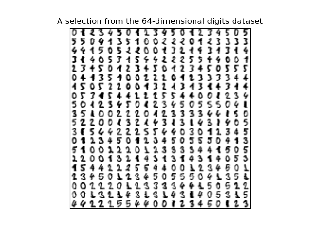
High-dimensional datasets can be very difficult to visualize. While data
in two or three dimensions can be plotted to show the inherent
structure of the data, equivalent high-dimensional plots are much less
intuitive. To aid visualization of the structure of a dataset, the
dimension must be reduced in some way.

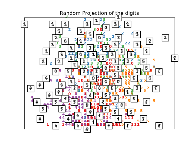
The simplest way to accomplish this dimensionality reduction is by taking
a random projection of the data. Though this allows some degree of
visualization of the data structure, the randomness of the choice leaves much
to be desired. In a random projection, it is likely that the more
interesting structure within the data will be lost.

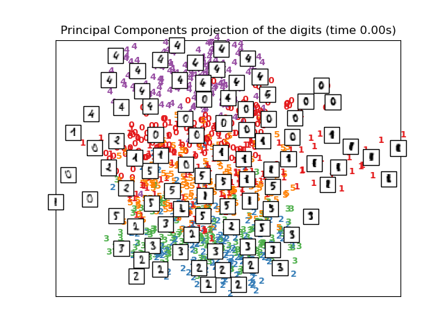
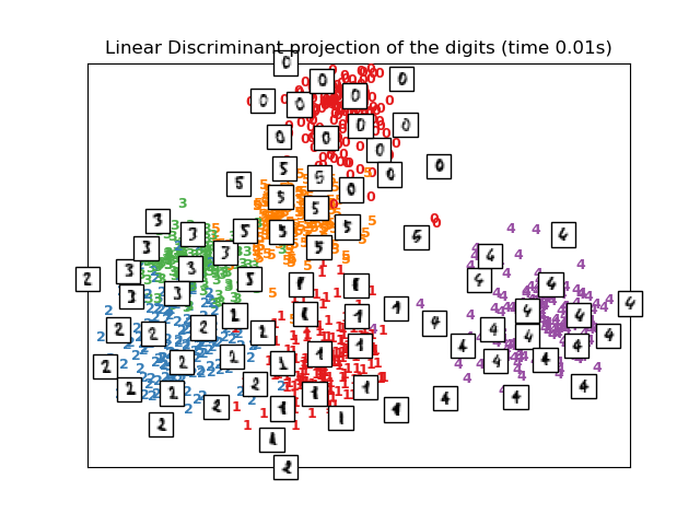
To address this concern, a number of supervised and unsupervised linear
dimensionality reduction frameworks have been designed, such as Principal
Component Analysis (PCA), Independent Component Analysis, Linear
Discriminant Analysis, and others. These algorithms define specific
rubrics to choose an “interesting” linear projection of the data.
These methods can be powerful, but often miss important non-linear
structure in the data.

Manifold Learning can be thought of as an attempt to generalize linear
frameworks like PCA to be sensitive to non-linear structure in data. Though
supervised variants exist, the typical manifold learning problem is
unsupervised: it learns the high-dimensional structure of the data
from the data itself, without the use of predetermined classifications.

Examples:

• See for an example of
  dimensionality reduction on handwritten digits.

• See for an example of
  dimensionality reduction on a toy “S-curve” dataset.

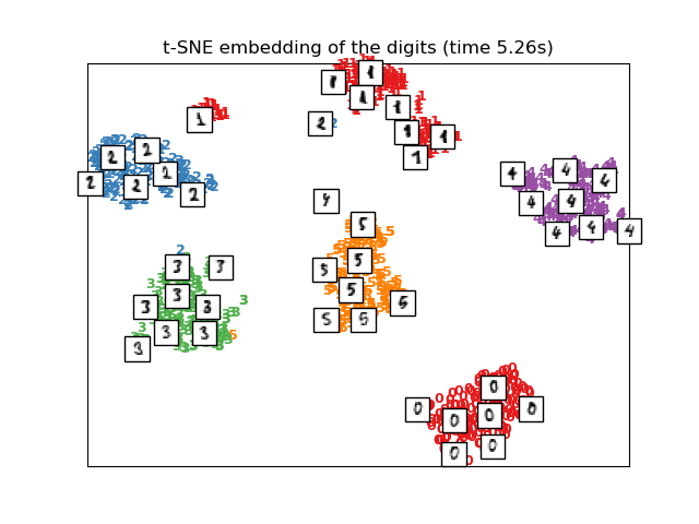
2.2.9. t-distributed Stochastic Neighbor Embedding (t-SNE)¶

t-SNE () converts affinities of data points to probabilities.
The affinities in the original space are represented by Gaussian joint
probabilities and the affinities in the embedded space are represented by
Student’s t-distributions. This allows t-SNE to be particularly sensitive
to local structure and has a few other advantages over existing techniques:

• Revealing the structure at many scales on a single map

• Revealing data that lie in multiple, different, manifolds or clusters

• Reducing the tendency to crowd points together at the center

While Isomap, LLE and variants are best suited to unfold a single continuous
low dimensional manifold, t-SNE will focus on the local structure of the data
and will tend to extract clustered local groups of samples as highlighted on
the S-curve example. This ability to group samples based on the local structure
might be beneficial to visually disentangle a dataset that comprises several
manifolds at once as is the case in the digits dataset.

The Kullback-Leibler (KL) divergence of the joint
probabilities in the original space and the embedded space will be minimized
by gradient descent. Note that the KL divergence is not convex, i.e.
multiple restarts with different initializations will end up in local minima
of the KL divergence. Hence, it is sometimes useful to try different seeds
and select the embedding with the lowest KL divergence.

The disadvantages to using t-SNE are roughly:

• t-SNE is computationally expensive, and can take several hours on million-sample
  datasets where PCA will finish in seconds or minutes

• The Barnes-Hut t-SNE method is limited to two or three dimensional embeddings.

• The algorithm is stochastic and multiple restarts with different seeds can
  yield different embeddings. However, it is perfectly legitimate to pick the
  embedding with the least error.

• Global structure is not explicitly preserved. This problem is mitigated by
  initializing points with PCA (using ).

2.2.9.1. Optimizing t-SNE

The main purpose of t-SNE is visualization of high-dimensional data. Hence,
it works best when the data will be embedded on two or three dimensions.

Optimizing the KL divergence can be a little bit tricky sometimes. There are
five parameters that control the optimization of t-SNE and therefore possibly
the quality of the resulting embedding:

• perplexity

• early exaggeration factor

• learning rate

• maximum number of iterations

• angle (not used in the exact method)

The perplexity is defined as \(k=2^{(S)}\) where \(S\) is the Shannon
entropy of the conditional probability distribution. The perplexity of a
\(k\)-sided die is \(k\), so that \(k\) is effectively the number of
nearest neighbors t-SNE considers when generating the conditional probabilities.
Larger perplexities lead to more nearest neighbors and less sensitive to small
structure. Conversely a lower perplexity considers a smaller number of
neighbors, and thus ignores more global information in favour of the
local neighborhood. As dataset sizes get larger more points will be
required to get a reasonable sample of the local neighborhood, and hence
larger perplexities may be required. Similarly noisier datasets will require
larger perplexity values to encompass enough local neighbors to see beyond
the background noise.

The maximum number of iterations is usually high enough and does not need
any tuning. The optimization consists of two phases: the early exaggeration
phase and the final optimization. During early exaggeration the joint
probabilities in the original space will be artificially increased by
multiplication with a given factor. Larger factors result in larger gaps
between natural clusters in the data. If the factor is too high, the KL
divergence could increase during this phase. Usually it does not have to be
tuned. A critical parameter is the learning rate. If it is too low gradient
descent will get stuck in a bad local minimum. If it is too high the KL
divergence will increase during optimization. More tips can be found in
Laurens van der Maaten’s FAQ (see references). The last parameter, angle,
is a tradeoff between performance and accuracy. Larger angles imply that we
can approximate larger regions by a single point, leading to better speed
but less accurate results.

“How to Use t-SNE Effectively”
provides a good discussion of the effects of the various parameters, as well
as interactive plots to explore the effects of different parameters.

Evaluation of the performance on the test set¶

Evaluating the predictive accuracy of the model is equally easy:

>>> import numpy as np
>>> twenty_test = fetch_20newsgroups(subset='test',
...     categories=categories, shuffle=True, random_state=42)
>>> docs_test = twenty_test.data
>>> predicted = text_clf.predict(docs_test)
>>> np.mean(predicted == twenty_test.target)
0.8348...

We achieved 83.5% accuracy. Let’s see if we can do better with a
linear ,
which is widely regarded as one of
the best text classification algorithms (although it’s also a bit slower
than naïve Bayes). We can change the learner by simply plugging a different
classifier object into our pipeline:

>>> from sklearn.linear_model import SGDClassifier
>>> text_clf = Pipeline()

>>> text_clf.fit(twenty_train.data, twenty_train.target)
Pipeline(...)
>>> predicted = text_clf.predict(docs_test)
>>> np.mean(predicted == twenty_test.target)
0.9101...

We achieved 91.3% accuracy using the SVM. provides further
utilities for more detailed performance analysis of the results:

>>> from sklearn import metrics
>>> print(metrics.classification_report(twenty_test.target, predicted,
...     target_names=twenty_test.target_names))
                        precision    recall  f1-score   support

           alt.atheism       0.95      0.80      0.87       319
         comp.graphics       0.87      0.98      0.92       389
               sci.med       0.94      0.89      0.91       396
soc.religion.christian       0.90      0.95      0.93       398

              accuracy                           0.91      1502
             macro avg       0.91      0.91      0.91      1502
          weighted avg       0.91      0.91      0.91      1502


>>> metrics.confusion_matrix(twenty_test.target, predicted)
array(,
       ,
       ,
       ])

1.12.7. Classifier Chain¶

Classifier chains (see ) are a way of combining a
number of binary classifiers into a single multi-label model that is capable
of exploiting correlations among targets.

For a multi-label classification problem with N classes, N binary
classifiers are assigned an integer between 0 and N-1. These integers
define the order of models in the chain. Each classifier is then fit on the
available training data plus the true labels of the classes whose
models were assigned a lower number.

When predicting, the true labels will not be available. Instead the
predictions of each model are passed on to the subsequent models in the
chain to be used as features.

Clearly the order of the chain is important. The first model in the chain
has no information about the other labels while the last model in the chain
has features indicating the presence of all of the other labels. In general
one does not know the optimal ordering of the models in the chain so
typically many randomly ordered chains are fit and their predictions are
averaged together.

Linear model: from regression to sparsity¶

Diabetes dataset

The diabetes dataset consists of 10 physiological variables (age,
sex, weight, blood pressure) measure on 442 patients, and an
indication of disease progression after one year:

>>> diabetes_X, diabetes_y = datasets.load_diabetes(return_X_y=True)
>>> diabetes_X_train = diabetes_X
>>> diabetes_y_train = diabetes_y

The task at hand is to predict disease progression from physiological
variables.

Linear regression

,
in its simplest form, fits a linear model to the data set by adjusting
a set of parameters in order to make the sum of the squared residuals
of the model as small as possible.

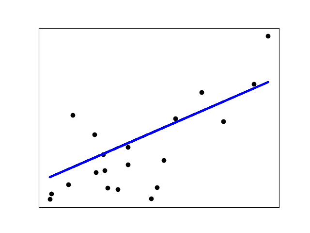
Linear models: \(y = X\beta + \epsilon\)

>>> from sklearn import linear_model
>>> regr = linear_model.LinearRegression()
>>> regr.fit(diabetes_X_train, diabetes_y_train)
LinearRegression()
>>> print(regr.coef_)  



>>> # The mean square error
>>> np.mean((regr.predict(diabetes_X_test) - diabetes_y_test)**2)
2004.56760268...

>>> # Explained variance score: 1 is perfect prediction
>>> # and 0 means that there is no linear relationship
>>> # between X and y.
>>> regr.score(diabetes_X_test, diabetes_y_test)
0.5850753022690...

Shrinkage

If there are few data points per dimension, noise in the observations
induces high variance:

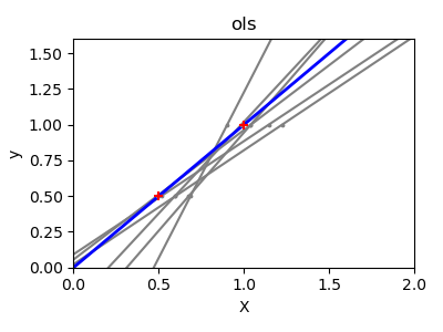
>>> X = np.c_ .5, 1.T
>>> y = .5, 1
>>> test = np.c_ , 2.T
>>> regr = linear_model.LinearRegression()

>>> import matplotlib.pyplot as plt 
>>> plt.figure() 

>>> np.random.seed()
>>> for _ in range(6): 
...     this_X = .1 * np.random.normal(size=(2, 1)) + X
...     regr.fit(this_X, y)
...     plt.plot(test, regr.predict(test)) 
...     plt.scatter(this_X, y, s=3)  

A solution in high-dimensional statistical learning is to shrink the
regression coefficients to zero: any two randomly chosen set of
observations are likely to be uncorrelated. This is called
regression:

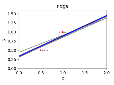
>>> regr = linear_model.Ridge(alpha=.1)

>>> plt.figure() 

>>> np.random.seed()
>>> for _ in range(6): 
...     this_X = .1 * np.random.normal(size=(2, 1)) + X
...     regr.fit(this_X, y)
...     plt.plot(test, regr.predict(test)) 
...     plt.scatter(this_X, y, s=3) 

This is an example of bias/variance tradeoff: the larger the ridge
parameter, the higher the bias and the lower the variance.

We can choose to minimize left out error, this time using the
diabetes dataset rather than our synthetic data:

>>> alphas = np.logspace(-4, -1, 6)
>>> print()

Note

Capturing in the fitted parameters noise that prevents the model to
generalize to new data is called
overfitting. The bias introduced
by the ridge regression is called a
regularization.

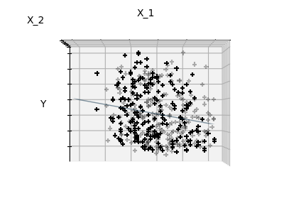
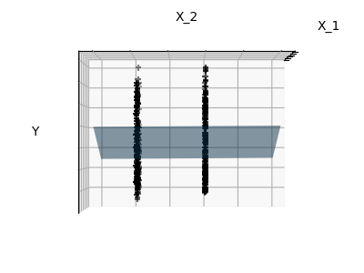
Sparsity

Fitting only features 1 and 2

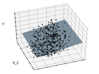
Note

A representation of the full diabetes dataset would involve 11
dimensions (10 feature dimensions and one of the target variable). It
is hard to develop an intuition on such representation, but it may be
useful to keep in mind that it would be a fairly empty space.

We can see that, although feature 2 has a strong coefficient on the full
model, it conveys little information on when considered with feature 1.

To improve the conditioning of the problem (i.e. mitigating the
), it would be interesting to select only the
informative features and set non-informative ones, like feature 2 to 0. Ridge
regression will decrease their contribution, but not set them to zero. Another
penalization approach, called (least absolute shrinkage and
selection operator), can set some coefficients to zero. Such methods are
called sparse method and sparsity can be seen as an
application of Occam’s razor: prefer simpler models.

>>> regr = linear_model.Lasso()
>>> scores = regr.set_params(alpha=alpha)
...               .fit(diabetes_X_train, diabetes_y_train)
...               .score(diabetes_X_test, diabetes_y_test)
...           for alpha in alphas
>>> best_alpha = alphasscores.index(max(scores))]
>>> regr.alpha = best_alpha
>>> regr.fit(diabetes_X_train, diabetes_y_train)
Lasso(alpha=0.025118864315095794)
>>> print(regr.coef_)

Different algorithms for the same problem

Different algorithms can be used to solve the same mathematical
problem. For instance the object in scikit-learn
solves the lasso regression problem using a
coordinate descent method,
that is efficient on large datasets. However, scikit-learn also
provides the object using the LARS algorithm,
which is very efficient for problems in which the weight vector estimated
is very sparse (i.e. problems with very few observations).

Interoperability and framework enhancements¶

These tools adapt scikit-learn for use with other technologies or otherwise
enhance the functionality of scikit-learn’s estimators.

Data formats

• Fast svmlight / libsvm file loader
  Fast and memory-efficient svmlight / libsvm file loader for Python.

• sklearn_pandas bridge for
  scikit-learn pipelines and pandas data frame with dedicated transformers.

• sklearn_xarray provides
  compatibility of scikit-learn estimators with xarray data structures.

Auto-ML

• auto-sklearn
  An automated machine learning toolkit and a drop-in replacement for a
  scikit-learn estimator

• TPOT
  An automated machine learning toolkit that optimizes a series of scikit-learn
  operators to design a machine learning pipeline, including data and feature
  preprocessors as well as the estimators. Works as a drop-in replacement for a
  scikit-learn estimator.

Experimentation frameworks

• REP Environment for conducting data-driven
  research in a consistent and reproducible way

• Scikit-Learn Laboratory A command-line
  wrapper around scikit-learn that makes it easy to run machine learning
  experiments with multiple learners and large feature sets.

Model inspection and visualisation

• dtreeviz A python library for
  decision tree visualization and model interpretation.

• eli5 A library for
  debugging/inspecting machine learning models and explaining their
  predictions.

• mlxtend Includes model visualization
  utilities.

• yellowbrick A suite of
  custom matplotlib visualizers for scikit-learn estimators to support visual feature
  analysis, model selection, evaluation, and diagnostics.

Model selection

• scikit-optimize
  A library to minimize (very) expensive and noisy black-box functions. It
  implements several methods for sequential model-based optimization, and
  includes a replacement for or to do
  cross-validated parameter search using any of these strategies.

• sklearn-deap Use evolutionary

  algorithms instead of gridsearch in scikit-learn.

Model export for production

1.10.7. Mathematical formulation¶

Given training vectors \(x_i \in R^n\), i=1,…, l and a label vector
\(y \in R^l\), a decision tree recursively partitions the space such
that the samples with the same labels are grouped together.

Let the data at node \(m\) be represented by \(Q\). For
each candidate split \(\theta = (j, t_m)\) consisting of a
feature \(j\) and threshold \(t_m\), partition the data into
\(Q_{left}(\theta)\) and \(Q_{right}(\theta)\) subsets

\

The impurity at \(m\) is computed using an impurity function
\(H()\), the choice of which depends on the task being solved
(classification or regression)

\

Select the parameters that minimises the impurity

\

Recurse for subsets \(Q_{left}(\theta^*)\) and
\(Q_{right}(\theta^*)\) until the maximum allowable depth is reached,
\(N_m < \min_{samples}\) or \(N_m = 1\).

1.10.7.1. Classification criteria

If a target is a classification outcome taking on values 0,1,…,K-1,
for node \(m\), representing a region \(R_m\) with \(N_m\)
observations, let

\[p_{mk} = 1/ N_m \sum_{x_i \in R_m} I(y_i = k)\]

be the proportion of class k observations in node \(m\)

Common measures of impurity are Gini

\

Entropy

\

and Misclassification

\

where \(X_m\) is the training data in node \(m\)

6.4.2. Univariate feature imputation¶

The class provides basic strategies for imputing missing
values. Missing values can be imputed with a provided constant value, or using
the statistics (mean, median or most frequent) of each column in which the
missing values are located. This class also allows for different missing values
encodings.

The following snippet demonstrates how to replace missing values,
encoded as , using the mean value of the columns (axis 0)
that contain the missing values:

>>> import numpy as np
>>> from sklearn.impute import SimpleImputer
>>> imp = SimpleImputer(missing_values=np.nan, strategy='mean')
>>> imp.fit(, np.nan, 3], 7, 6]])
SimpleImputer()
>>> X = , 6, np.nan], 7, 6]]
>>> print(imp.transform(X))

 
 ]

The class also supports sparse matrices:

>>> import scipy.sparse as sp
>>> X = sp.csc_matrix(, , -1], 8, 4]])
>>> imp = SimpleImputer(missing_values=-1, strategy='mean')
>>> imp.fit(X)
SimpleImputer(missing_values=-1)
>>> X_test = sp.csc_matrix(, 6, -1], 7, 6]])
>>> print(imp.transform(X_test).toarray())

 
 ]

Note that this format is not meant to be used to implicitly store missing
values in the matrix because it would densify it at transform time. Missing
values encoded by 0 must be used with dense input.

The class also supports categorical data represented as
string values or pandas categoricals when using the or
strategy:

1.9.3. Complement Naive Bayes¶

implements the complement naive Bayes (CNB) algorithm.
CNB is an adaptation of the standard multinomial naive Bayes (MNB) algorithm
that is particularly suited for imbalanced data sets. Specifically, CNB uses
statistics from the complement of each class to compute the model’s weights.
The inventors of CNB show empirically that the parameter estimates for CNB are
more stable than those for MNB. Further, CNB regularly outperforms MNB (often
by a considerable margin) on text classification tasks. The procedure for
calculating the weights is as follows:

\

where the summations are over all documents \(j\) not in class \(c\),
\(d_{ij}\) is either the count or tf-idf value of term \(i\) in document
\(j\), \(\alpha_i\) is a smoothing hyperparameter like that found in
MNB, and \(\alpha = \sum_{i} \alpha_i\). The second normalization addresses
the tendency for longer documents to dominate parameter estimates in MNB. The
classification rule is:

\

i.e., a document is assigned to the class that is the poorest complement
match.

3.2.3. Tips for parameter search¶

3.2.3.1. Specifying an objective metric

By default, parameter search uses the function of the estimator
to evaluate a parameter setting. These are the
for classification and
for regression. For some applications,
other scoring functions are better suited (for example in unbalanced
classification, the accuracy score is often uninformative). An alternative
scoring function can be specified via the parameter to
, and many of the
specialized cross-validation tools described below.
See for more details.

3.2.3.2. Specifying multiple metrics for evaluation

and allow specifying multiple metrics
for the parameter.

Multimetric scoring can either be specified as a list of strings of predefined
scores names or a dict mapping the scorer name to the scorer function and/or
the predefined scorer name(s). See for more details.

When specifying multiple metrics, the parameter must be set to the
metric (string) for which the will be found and used to build
the on the whole dataset. If the search should not be
refit, set . Leaving refit to the default value will
result in an error when using multiple metrics.

See
for an example usage.

3.2.3.3. Composite estimators and parameter spaces

and allow searching over
parameters of composite or nested estimators such as
,
,
or
using a dedicated
syntax:

>>> from sklearn.model_selection import GridSearchCV
>>> from sklearn.calibration import CalibratedClassifierCV
>>> from sklearn.ensemble import RandomForestClassifier
>>> from sklearn.datasets import make_moons
>>> X, y = make_moons()
>>> calibrated_forest = CalibratedClassifierCV(
...    base_estimator=RandomForestClassifier(n_estimators=10))
>>> param_grid = {
...    'base_estimator__max_depth' 2, 4, 6, 8]}
>>> search = GridSearchCV(calibrated_forest, param_grid, cv=5)
>>> search.fit(X, y)
GridSearchCV(cv=5,
             estimator=CalibratedClassifierCV(...),
             param_grid={'base_estimator__max_depth': })

Here, is the parameter name of the nested estimator,
in this case .
If the meta-estimator is constructed as a collection of estimators as in
, then refers to the name of the estimator,
see . In practice, there can be several
levels of nesting:

>>> from sklearn.pipeline import Pipeline
>>> from sklearn.feature_selection import SelectKBest
>>> pipe = Pipeline()
>>> param_grid = {
...    'select__k' 1, 2],
...    'model__base_estimator__max_depth' 2, 4, 6, 8]}
>>> search = GridSearchCV(pipe, param_grid, cv=5).fit(X, y)

3.2.3.4. Model selection: development and evaluation

Model selection by evaluating various parameter settings can be seen as a way
to use the labeled data to “train” the parameters of the grid.

When evaluating the resulting model it is important to do it on
held-out samples that were not seen during the grid search process:
it is recommended to split the data into a development set (to
be fed to the instance) and an evaluation set
to compute performance metrics.

This can be done by using the
utility function.

3.2.3.5. Parallelism

and evaluate each parameter
setting independently. Computations can be run in parallel if your OS
supports it, by using the keyword . See function signature for
more details.

1.13.4. Feature selection using SelectFromModel¶

is a meta-transformer that can be used along with any
estimator that has a or attribute after fitting.
The features are considered unimportant and removed, if the corresponding
or values are below the provided
parameter. Apart from specifying the threshold numerically,
there are built-in heuristics for finding a threshold using a string argument.
Available heuristics are “mean”, “median” and float multiples of these like
“0.1*mean”. In combination with the criteria, one can use the
parameter to set a limit on the number of features to select.

For examples on how it is to be used refer to the sections below.

Examples

Feature selection using SelectFromModel and LassoCV: Selecting the two
most important features from the diabetes dataset without knowing the
threshold beforehand.

1.13.4.1. L1-based feature selection

penalized with the L1 norm have
sparse solutions: many of their estimated coefficients are zero. When the goal
is to reduce the dimensionality of the data to use with another classifier,
they can be used along with
to select the non-zero coefficients. In particular, sparse estimators useful
for this purpose are the for regression, and
of and
for classification:

>>> from sklearn.svm import LinearSVC
>>> from sklearn.datasets import load_iris
>>> from sklearn.feature_selection import SelectFromModel
>>> X, y = load_iris(return_X_y=True)
>>> X.shape
(150, 4)
>>> lsvc = LinearSVC(C=0.01, penalty="l1", dual=False).fit(X, y)
>>> model = SelectFromModel(lsvc, prefit=True)
>>> X_new = model.transform(X)
>>> X_new.shape
(150, 3)

With SVMs and logistic-regression, the parameter C controls the sparsity:
the smaller C the fewer features selected. With Lasso, the higher the
alpha parameter, the fewer features selected.

Examples:

Classification of text documents using sparse features: Comparison
of different algorithms for document classification including L1-based
feature selection.

L1-recovery and compressive sensing

For a good choice of alpha, the can fully recover the
exact set of non-zero variables using only few observations, provided
certain specific conditions are met. In particular, the number of
samples should be “sufficiently large”, or L1 models will perform at
random, where “sufficiently large” depends on the number of non-zero
coefficients, the logarithm of the number of features, the amount of
noise, the smallest absolute value of non-zero coefficients, and the
structure of the design matrix X. In addition, the design matrix must
display certain specific properties, such as not being too correlated.

There is no general rule to select an alpha parameter for recovery of
non-zero coefficients. It can by set by cross-validation
( or ), though this may lead to
under-penalized models: including a small number of non-relevant
variables is not detrimental to prediction score. BIC
() tends, on the opposite, to set high values of
alpha.

Reference Richard G. Baraniuk “Compressive Sensing”, IEEE Signal
Processing Magazine July 2007
http://users.isr.ist.utl.pt/~aguiar/CS_notes.pdf

Third party distributions of scikit-learn¶

Some third-party distributions provide versions of
scikit-learn integrated with their package-management systems.

These can make installation and upgrading much easier for users since
the integration includes the ability to automatically install
dependencies (numpy, scipy) that scikit-learn requires.

The following is an incomplete list of OS and python distributions
that provide their own version of scikit-learn.

Arch Linux

Arch Linux’s package is provided through the official repositories as
for Python.
It can be installed by typing the following command:

$ sudo pacman -S python-scikit-learn

Debian/Ubuntu

The Debian/Ubuntu package is splitted in three different packages called
(python modules), (low-level
implementations and bindings), (documentation).
Only the Python 3 version is available in the Debian Buster (the more recent
Debian distribution).
Packages can be installed using :

$ sudo apt-get install python3-sklearn python3-sklearn-lib python3-sklearn-doc

Fedora

The Fedora package is called for the python 3 version,
the only one available in Fedora30.
It can be installed using :

$ sudo dnf install python3-scikit-learn

MacPorts for Mac OSX

The MacPorts package is named ,
where denotes the Python version.
It can be installed by typing the following
command:

$ sudo port install py36-scikit-learn

Canopy and Anaconda for all supported platforms

Canopy and Anaconda both ship a recent
version of scikit-learn, in addition to a large set of scientific python
library for Windows, Mac OSX and Linux.

Anaconda offers scikit-learn as part of its free distribution.

Intel conda channel

Intel maintains a dedicated conda channel that ships scikit-learn:

$ conda install -c intel scikit-learn

This version of scikit-learn comes with alternative solvers for some common
estimators. Those solvers come from the DAAL C++ library and are optimized for
multi-core Intel CPUs.

Note that those solvers are not enabled by default, please refer to the
daal4py documentation
for more details.

Compatibility with the standard scikit-learn solvers is checked by running the
full scikit-learn test suite via automated continuous integration as reported
on https://github.com/IntelPython/daal4py.

1.10.6. Tree algorithms: ID3, C4.5, C5.0 and CART¶

What are all the various decision tree algorithms and how do they differ
from each other? Which one is implemented in scikit-learn?

ID3 (Iterative Dichotomiser 3) was developed in 1986 by Ross Quinlan.
The algorithm creates a multiway tree, finding for each node (i.e. in
a greedy manner) the categorical feature that will yield the largest
information gain for categorical targets. Trees are grown to their
maximum size and then a pruning step is usually applied to improve the
ability of the tree to generalise to unseen data.

C4.5 is the successor to ID3 and removed the restriction that features
must be categorical by dynamically defining a discrete attribute (based
on numerical variables) that partitions the continuous attribute value
into a discrete set of intervals. C4.5 converts the trained trees
(i.e. the output of the ID3 algorithm) into sets of if-then rules.
These accuracy of each rule is then evaluated to determine the order
in which they should be applied. Pruning is done by removing a rule’s
precondition if the accuracy of the rule improves without it.

C5.0 is Quinlan’s latest version release under a proprietary license.
It uses less memory and builds smaller rulesets than C4.5 while being
more accurate.

(Classification and Regression Trees) is very similar to C4.5, but
it differs in that it supports numerical target variables (regression) and
does not compute rule sets. CART constructs binary trees using the feature
and threshold that yield the largest information gain at each node.

1.13.3. Recursive feature elimination¶

Given an external estimator that assigns weights to features (e.g., the
coefficients of a linear model), recursive feature elimination ()
is to select features by recursively considering smaller and smaller sets of
features. First, the estimator is trained on the initial set of features and
the importance of each feature is obtained either through a attribute
or through a attribute. Then, the least important
features are pruned from current set of features.That procedure is recursively
repeated on the pruned set until the desired number of features to select is
eventually reached.

performs RFE in a cross-validation loop to find the optimal
number of features.

6.4.3. Multivariate feature imputation¶

A more sophisticated approach is to use the class,
which models each feature with missing values as a function of other features,
and uses that estimate for imputation. It does so in an iterated round-robin
fashion: at each step, a feature column is designated as output and the
other feature columns are treated as inputs . A regressor is fit on for known . Then, the regressor is used to predict the missing values
of . This is done for each feature in an iterative fashion, and then is
repeated for imputation rounds. The results of the final
imputation round are returned.

Note

This estimator is still experimental for now: default parameters or
details of behaviour might change without any deprecation cycle. Resolving
the following issues would help stabilize :
convergence criteria (#14338), default estimators (#13286),
and use of random state (#15611). To use it, you need to explicitly
import .

>>> import numpy as np
>>> from sklearn.experimental import enable_iterative_imputer
>>> from sklearn.impute import IterativeImputer
>>> imp = IterativeImputer(max_iter=10, random_state=)
>>> imp.fit(, 3, 6], 4, 8], np.nan, 3], 7, np.nan]])
IterativeImputer(random_state=0)
>>> X_test = , 6, np.nan], np.nan, 6]]
>>> # the model learns that the second feature is double the first
>>> print(np.round(imp.transform(X_test)))

 
 ]

Both and can be used in a
Pipeline as a way to build a composite estimator that supports imputation.
See .

6.4.3.1. Flexibility of IterativeImputer

There are many well-established imputation packages in the R data science
ecosystem: Amelia, mi, mice, missForest, etc. missForest is popular, and turns
out to be a particular instance of different sequential imputation algorithms
that can all be implemented with by passing in
different regressors to be used for predicting missing feature values. In the
case of missForest, this regressor is a Random Forest.
See .

6.2.2. Feature hashing¶

The class is a high-speed, low-memory vectorizer that
uses a technique known as
feature hashing,
or the “hashing trick”.
Instead of building a hash table of the features encountered in training,
as the vectorizers do, instances of
apply a hash function to the features
to determine their column index in sample matrices directly.
The result is increased speed and reduced memory usage,
at the expense of inspectability;
the hasher does not remember what the input features looked like
and has no method.

Since the hash function might cause collisions between (unrelated) features,
a signed hash function is used and the sign of the hash value
determines the sign of the value stored in the output matrix for a feature.
This way, collisions are likely to cancel out rather than accumulate error,
and the expected mean of any output feature’s value is zero. This mechanism
is enabled by default with and is particularly useful
for small hash table sizes (). For large hash table
sizes, it can be disabled, to allow the output to be passed to estimators like
or

feature selectors that expect non-negative inputs.

accepts either mappings
(like Python’s and its variants in the module),
pairs, or strings,
depending on the constructor parameter .
Mapping are treated as lists of pairs,
while single strings have an implicit value of 1,
so is interpreted as
.
If a single feature occurs multiple times in a sample,
the associated values will be summed
(so and become ).
The output from is always a matrix
in the CSR format.

Feature hashing can be employed in document classification,
but unlike ,
does not do word
splitting or any other preprocessing except Unicode-to-UTF-8 encoding;
see , below, for a combined tokenizer/hasher.

As an example, consider a word-level natural language processing task
that needs features extracted from pairs.
One could use a Python generator function to extract features:

def token_features(token, part_of_speech):
    if token.isdigit():
        yield "numeric"
    else
        yield "token={}".format(token.lower())
        yield "token,pos={},{}".format(token, part_of_speech)
    if token.isupper():
        yield "uppercase_initial"
    if token.isupper():
        yield "all_uppercase"
    yield "pos={}".format(part_of_speech)

Then, the to be fed to
can be constructed using:

raw_X = (token_features(tok, pos_tagger(tok)) for tok in corpus)

and fed to a hasher with:

hasher = FeatureHasher(input_type='string')
X = hasher.transform(raw_X)

to get a matrix .

Note the use of a generator comprehension,
which introduces laziness into the feature extraction:
tokens are only processed on demand from the hasher.