Corpus readers and custom corpora
Содержание:
- Sentence Detection#
- nltk.classify.rte_classify module
- Линейная регрессия с одной независимой переменной
- Stop Words#
- Морфологический анализ
- nltk.classify.positivenaivebayes module
- nltk.lm.models module
- nltk.classify.weka module
- nltk.classify.api module
- Линейная регрессия с несколькими переменными в Scikit-learn
- nlp prediction example
- nltk.classify.scikitlearn module
- Терминология NLP
- Lemmatization#
- nltk.classify.util module
- История
- Интегрированные пакеты
- nltk.metrics.segmentation module
- Tokenization in spaCy#
- nltk.metrics.aline module
Sentence Detection#
Sentence Detection is the process of locating the start and end of sentences in a given text. This allows you to you divide a text into linguistically meaningful units. You’ll use these units when you’re processing your text to perform tasks such as part of speech tagging and entity extraction.
In spaCy, the property is used to extract sentences. Here’s how you would extract the total number of sentences and the sentences for a given input text:
>>>
In the above example, spaCy is correctly able to identify sentences in the English language, using a full stop() as the sentence delimiter. You can also customize the sentence detection to detect sentences on custom delimiters.
Here’s an example, where an ellipsis() is used as the delimiter:
>>>
Note that contain three sentences, whereas contains two sentences. These sentences are still obtained via the attribute, as you saw before.
nltk.classify.rte_classify module
Simple classifier for RTE corpus.
It calculates the overlap in words and named entities between text and
hypothesis, and also whether there are words / named entities in the
hypothesis which fail to occur in the text, since this is an indicator that
the hypothesis is more informative than (i.e not entailed by) the text.
TO DO: better Named Entity classification
TO DO: add lemmatization
- class (rtepair, stop=True, use_lemmatize=False)
-
Bases:
This builds a bag of words for both the text and the hypothesis after
throwing away some stopwords, then calculates overlap and difference.- (toktype, debug=True)
-
Compute the extraneous material in the hypothesis.
- Parameters
-
toktype (‘ne’ or ‘word’) – distinguish Named Entities from ordinary words
- (toktype, debug=False)
-
Compute the overlap between text and hypothesis.
- Parameters
-
toktype (‘ne’ or ‘word’) – distinguish Named Entities from ordinary words
- (algorithm)
- (rtepair)
Линейная регрессия с одной независимой переменной
Графически линейная регрессия с одной независимой выглядит как прямая. Она решает задачу регрессии нахождением прямой, которая наилучшим образом соответствует точкам наблюдений. Следующий рисунок иллюстрирует вышесказанное:
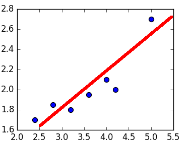 Линейная регрессия (красная линия) наиболее полно соответствует точкам
Модель линейной регрессии может быть задана следующим образом:
Следовательно, для решения задачи регрессии требуется найти коэффициенты (коэффициент наклона) и (точка пересечения линии с осью ординат). Не вдаваясь в подробности, их можно выразить так:
Найдем коэффициенты в Python, написав следующие функции:
def calculate_slope(x, y):
    mx = x - x.mean()
    my = y - y.mean()
    return sum(mx * my) / sum(mx**2)

def get_params(x, y):
    a = calculate_slope(x, y)
    b = y.mean() - a * x.mean()
    return a, b
Стоит заметить, функция сначала находит произведение двух массивов, только потом суммирует результат этого произведения.
В нашем случае выберем в качестве независимой переменной – количество отзывов , a зависимой переменной , которую требуется предсказать, будет цена . Кроме того, чтобы избежать излишней волатильности цены, мы ее прологарифмируем, как это объяснялось в прошлый раз. Посмотрим на полученные коэффициенты:
>>> import numpy as np
import numpy as np
d = data
x = d.number_of_reviews
y = np.log(d.price)
a, b = get_params(x, y)
В итоге получили:
>>> a
-0.04213862786693919
>>> b
125.40308200933784
Мы отфильтровали нулевые значения цены, так как логарифма от нуля не существует. Таким образом, линейная регрессия будет задаваться как:
Построим график в Python-библиотеке matplotlib, на котором будет видна полученная линейная регрессия и истинные значения цены. О том, как строить графики, мы рассказывали тут. Для этого воспользуемся функциями и :
import matplotlib.pyplot as plt

plt.xlabel('Количество отзывов')
plt.ylabel('Цена в логарифмическом масштабе')
plt.scatter(x, y)
plt.plot(x, lin_reg, color='red')
В результате получили график:
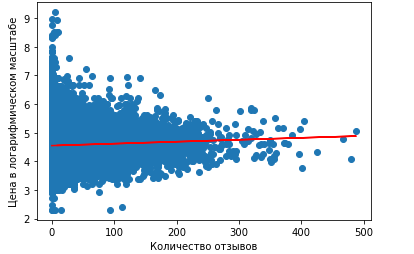 Линейная регрессия (красная линия)
Как можно заметить, линейная регрессия с одной независимой переменной показывает неудачные результаты, так как является практически параллельной оси абсцисс. Поэтому предсказание будет одним и тем же, примерно равным 4.6. При переводе обратно в нормальный масштаб равняется $100.
Stop Words#
Stop words are the most common words in a language. In the English language, some examples of stop words are , , , and . Most sentences need to contain stop words in order to be full sentences that make sense.
Generally, stop words are removed because they aren’t significant and distort the word frequency analysis. spaCy has a list of stop words for the English language:
>>>
You can remove stop words from the input text:
>>>
Stop words like , , , , and are not printed in the output above. You can also create a list of tokens not containing stop words:
>>>
can be joined with spaces to form a sentence with no stop words.
Морфологический анализ
| Название | Метод | Языки | Лицензия | Платформа |
|---|---|---|---|---|
| словарный | русский, английский, немецкий | LGPL | Linux, Windows | |
| Snowball | алгоритм Портера | русский, английский | BSD | Linux, Windows |
| Stemka | словарный | русский | Собственная | Linux, Windows |
| pymorphy | словарный | русский, английский, немецкий | MIT | Python |
| Myaso | алгоритм Витерби | русский, английский | MIT | Ruby |
| Eureka Engine | машинное обучение | русский | Коммерческая | Веб-сервис |
| машинное обучение | русский, английский | Бесплатная для исследовательских целей + коммерческая | Веб-сервис, Java, Python | |
| русский, английский | LGPLv3 + некоммерческая | Python, C++ | ||
| словарный | русский, английский, немецкий | LGPL | PHP | |
| словарный | русский, английский, украинский | Non-Commercial Freeware | .NET, .NET Core, Java и Python | |
| FreeLing | словарный | русский, англиский, итальянский, испанский, португальский, астурийский, валийский, галисийский, каталанский | GPL + Коммерческая | Linux |
| машинное обучение | английский | Apache License | Python | |
| машинное обучение | английский | MIT | Python | |
| машинное обучение | английский | GPL | Python | |
| правила, регулярные выражения | английский, испанский, немецкий, французский, итальянский, нидерландский | BSD | Python | |
| правила | английский, французский, японский | MIT | Node.js | |
| словарный | русский, английский | MIT | Linux | |
| алгоритм Витерби | английский, корейский | BSD | Linux, Windows | |
| метод опорных векторов | русский, английский | LGPL | Perl | |
| машинное обучение | английский | GPL | Java | |
| машинное обучение | английский, немецкий, арабский, китайский | GPL | Java | |
| словарный | русский | Apache License | Java | |
| словарный | русский | GPL | Java | |
| mystem | словарный | русский | Некоммерческая | Linux, Windows |
| TreeTagger | деревья принятия решений | русский, английский, немецкий, французский, итальянский, нидерландский, испанский, болгарский, греческий, португальский, китайский, суахили, латинский, эстонский | Некоммерческая | Linux, Windows |
| алгоритм Витерби | русский, английский | Некоммерческая | Linux | |
| словарный | русский, украинский | Коммерческая | Windows, Веб-сервис | |
| словарный | русский | Коммерческая | Windows | |
| словарный, правила | русский, английский | Коммерческая | Windows | |
| словарный | русский, английский | Коммерческая | Linux, Windows | |
| словарный | русский, украинский, английский, французский, немецкий, испанский, итальянский, португальский | Коммерческая | Windows | |
| словарный | русский | н/д | Windows | |
| словарный | русский | MIT + некоммерческая | Java on Linux, Windows | |
| машинное обучение, словарный | русский | некоммерческая | .NET on Linux, Windows | |
| машинное обучение, словарный | английский | некоммерческая | .NET on Linux, Windows |
nltk.classify.positivenaivebayes module
A variant of the Naive Bayes Classifier that performs binary classification with
partially-labeled training sets. In other words, assume we want to build a classifier
that assigns each example to one of two complementary classes (e.g., male names and
female names).
If we have a training set with labeled examples for both classes, we can use a
standard Naive Bayes Classifier. However, consider the case when we only have labeled
examples for one of the classes, and other, unlabeled, examples.
Then, assuming a prior distribution on the two labels, we can use the unlabeled set
to estimate the frequencies of the various features.
Let the two possible labels be 1 and 0, and let’s say we only have examples labeled 1
and unlabeled examples. We are also given an estimate of P(1).
We compute P(feature|1) exactly as in the standard case.
To compute P(feature|0), we first estimate P(feature) from the unlabeled set (we are
assuming that the unlabeled examples are drawn according to the given prior distribution)
and then express the conditional probability as:
P(feature) — P(feature|1) * P(1)
P(feature|0) = ———————————-
P(0)
Example:
>>> from nltk.classify import PositiveNaiveBayesClassifier
Some sentences about sports:
>>> sports_sentences =  'The team dominated the game',
...                      'They lost the ball',
...                      'The game was intense',
...                      'The goalkeeper catched the ball',
...                      'The other team controlled the ball'
Mixed topics, including sports:
>>> various_sentences =  'The President did not comment',
...                       'I lost the keys',
...                       'The team won the game',
...                       'Sara has two kids',
...                       'The ball went off the court',
...                       'They had the ball for the whole game',
...                       'The show is over'
The features of a sentence are simply the words it contains:
>>> def features(sentence):
...     words = sentence.lower().split()
...     return dict(('contains(%s)' % w, True) for w in words)
We use the sports sentences as positive examples, the mixed ones ad unlabeled examples:
>>> positive_featuresets = map(features, sports_sentences)
>>> unlabeled_featuresets = map(features, various_sentences)
>>> classifier = PositiveNaiveBayesClassifier.train(positive_featuresets,
...                                                 unlabeled_featuresets)
Is the following sentence about sports?
>>> classifier.classify(features('The cat is on the table'))
False
What about this one?
>>> classifier.classify(features('My team lost the game'))
True
- class (label_probdist, feature_probdist)
-
Bases:
- static (positive_featuresets, unlabeled_featuresets, positive_prob_prior=0.5, estimator=<class ‘nltk.probability.ELEProbDist’>)
-
- Parameters
-
-
positive_featuresets – An iterable of featuresets that are known as positive
examples (i.e., their label is ). -
unlabeled_featuresets – An iterable of featuresets whose label is unknown.
-
positive_prob_prior – A prior estimate of the probability of the label
(default 0.5).
-
nltk.lm.models module
Language Models
- class (smoothing_cls, order, **kwargs)
-
Bases:
Logic common to all interpolated language models.
The idea to abstract this comes from Chen & Goodman 1995.
Do not instantiate this class directly!- (word, context=None)
-
Score a word given some optional context.
Concrete models are expected to provide an implementation.
Note that this method does not mask its arguments with the OOV label.
Use the score method for that.- Parameters
-
-
word (str) – Word for which we want the score
-
context (tuple(str)) – Context the word is in.
-
If None, compute unigram score.
:param context: tuple(str) or None
:rtype: float
- class (order, discount=0.1, **kwargs)
-
Bases:
Interpolated version of Kneser-Ney smoothing.
- class (*args, **kwargs)
-
Bases:
Implements Laplace (add one) smoothing.
Initialization identical to BaseNgramModel because gamma is always 1.
- class (gamma, *args, **kwargs)
-
Bases:
Provides Lidstone-smoothed scores.
In addition to initialization arguments from BaseNgramModel also requires
a number by which to increase the counts, gamma.- (word, context=None)
-
Add-one smoothing: Lidstone or Laplace.
To see what kind, look at gamma attribute on the class.
- class (order, vocabulary=None, counter=None)
-
Bases:
Class for providing MLE ngram model scores.
Inherits initialization from BaseNgramModel.
- (word, context=None)
-
Returns the MLE score for a word given a context.
Args:
— word is expcected to be a string
— context is expected to be something reasonably convertible to a tuple
nltk.classify.weka module
Classifiers that make use of the external ‘Weka’ package.
- class (labels, features)
-
Bases:
Converts featuresets and labeled featuresets to ARFF-formatted
strings, appropriate for input into Weka.Features and classes can be specified manually in the constructor, or may
be determined from data using .- (tokens, labeled=None)
-
Returns the ARFF data section for the given data.
- Parameters
-
-
tokens – a list of featuresets (dicts) or labelled featuresets
which are tuples (featureset, label). -
labeled – Indicates whether the given tokens are labeled
or not. If None, then the tokens will be assumed to be
labeled if the first token’s value is a tuple or list.
-
- (tokens)
-
Returns a string representation of ARFF output for the given data.
- static (tokens)
-
Constructs an ARFF_Formatter instance with class labels and feature
types determined from the given data. Handles boolean, numeric and
string (note: not nominal) types.
- ()
-
Returns an ARFF header as a string.
- ()
-
Returns the list of classes.
- (outfile, tokens)
-
Writes ARFF data to a file for the given data.
- class (formatter, model_filename)
-
Bases:
- (featuresets)
-
Apply to each element of . I.e.:
- Return type
-
list(label)
- (s)
- (lines)
- (featuresets)
-
Apply to each element of . I.e.:
- Return type
-
list()
- classmethod (model_filename, featuresets, classifier=’naivebayes’, options=[], quiet=True)
nltk.classify.api module
Interfaces for labeling tokens with category labels (or “class labels”).
is a standard interface for “single-category
classification”, in which the set of categories is known, the number
of categories is finite, and each text belongs to exactly one
category.
is a standard interface for “multi-category
classification”, which is like single-category classification except
that each text belongs to zero or more categories.
- class
-
Bases:
A processing interface for labeling tokens with a single category
label (or “class”). Labels are typically strs or
ints, but can be any immutable type. The set of labels
that the classifier chooses from must be fixed and finite.- Subclasses must define:
-
-
either or (or both)
-
- Subclasses may define:
- (featureset)
-
- Returns
-
the most appropriate label for the given featureset.
- Return type
-
label
- (featuresets)
-
Apply to each element of . I.e.:
- Return type
-
list(label)
- ()
-
- Returns
-
the list of category labels used by this classifier.
- Return type
-
list of (immutable)
- (featureset)
-
- Returns
-
a probability distribution over labels for the given
featureset. - Return type
- (featuresets)
-
Apply to each element of . I.e.:
- Return type
-
list()
Линейная регрессия с несколькими переменными в Scikit-learn
В действительности ML-модели редко обучаются только на одном признаке, что подтверждают построенные графики. Поэтому уравнение для линейной регрессии можно обобщить до переменных (признаков):
где задача сводится к нахождению коэффициентов. Не вдаваясь в подробности их нахождения, отметим, что Python-библиотека Scikit-learn предоставляет для этого уже готовый интерфейс.
Рассмотрим пример в Python. Выберем в качестве независимых переменных признаки: , , . Атрибут имеет Nan-значения, поэтому в дальнейшем заполним их нулями. К тому же, мы отфильтровали те данные, которые имеют нулевую цену:
d = data
d.fillna(0, inplace=True)

x = d.loc
y = d.loc
Здесь используется метод , который, согласно документации, быстрее и производительнее явного вызова столбцов []. Нам также требуется разбить полученные данные на тренировочную и тестовую выборки, чтобы на одних данных обучить модель, а на других – проверить ее корректность. В Scikit-learn имеется функция , возвращающая две пары массивов – тренировочного и тестового:
from sklearn.model_selection import train_test_split
x_train, x_test, y_train, y_test = train_test_split(x, y, test_size=0.2)
Данная функция принимает в качестве аргумента также , который определяет долю, отведенную на тестовую выборку.
Теперь к самому главному – обучению модели линейной регрессии. В Scikit-learn есть класс, который выполнит за нас работу в Python:
from sklearn.linear_model import LinearRegression
model = LinearRegression().fit(x_train, y_train)
В метод мы посылаем те данные, на которых ML-модель обучается. Попробуем получить предсказания на основе тестовой выборки:
y_pred = model.predict(x_test)
А как узнать, что такая модель лучшая из всех доступных? Нужно воспользоваться метриками качества.
nlp prediction example
Given a name, the classifier will predict if it’s a male or female.
To create our analysis program, we have several steps:
- Data preparation
- Feature extraction
- Training
- Prediction
Data preparation
The first step is to prepare data.
We use the names set included with nltk.
from nltk.corpus import names

# Load data and training
names = ((name, 'male') for name in names.words('male.txt') +
	 (name, 'female') for name in names.words('female.txt'))
|
This dataset is simply a collection of tuples. To give you an idea of what the dataset looks like:
(u'Aaron', 'male'), (u'Abbey', 'male'), (u'Abbie', 'male') (u'Zorana', 'female'), (u'Zorina', 'female'), (u'Zorine', 'female') |
You can define your own set of tuples if you wish, its simply a list containing many tuples.
Feature extraction
Based on the dataset, we prepare our feature. The feature we will use is the last letter of a name:
We define a featureset using:
featuresets = (gender_features(n), g) for (n,g) in names |
and the features (last letters) are extracted using:
def gender_features(word):
    return {'last_letter': word-1}
|
Training and prediction
We train and predict using:
classifier = nltk.NaiveBayesClassifier.train(train_set)

# Predict
print(classifier.classify(gender_features('Frank')))
|
Example
A classifier has a training and a test phrase.
import nltk.classify.util
from nltk.classify import NaiveBayesClassifier
from nltk.corpus import names

def gender_features(word):
    return {'last_letter': word-1}

# Load data and training
names = ((name, 'male') for name in names.words('male.txt') +
	 (name, 'female') for name in names.words('female.txt'))

featuresets = (gender_features(n), g) for (n,g) in names
train_set = featuresets
classifier = nltk.NaiveBayesClassifier.train(train_set)

# Predict
print(classifier.classify(gender_features('Frank')))
|
If you want to give the name during runtime, change the last line to:
# Predict
name = input("Name: ")
print(classifier.classify(gender_features(name)))
|
nltk.classify.scikitlearn module
scikit-learn (http://scikit-learn.org) is a machine learning library for
Python. It supports many classification algorithms, including SVMs,
Naive Bayes, logistic regression (MaxEnt) and decision trees.
This package implements a wrapper around scikit-learn classifiers. To use this
wrapper, construct a scikit-learn estimator object, then use that to construct
a SklearnClassifier. E.g., to wrap a linear SVM with default settings:
>>> from sklearn.svm import LinearSVC
>>> from nltk.classify.scikitlearn import SklearnClassifier
>>> classif = SklearnClassifier(LinearSVC())
A scikit-learn classifier may include preprocessing steps when it’s wrapped
in a Pipeline object. The following constructs and wraps a Naive Bayes text
classifier with tf-idf weighting and chi-square feature selection to get the
best 1000 features:
>>> from sklearn.feature_extraction.text import TfidfTransformer
>>> from sklearn.feature_selection import SelectKBest, chi2
>>> from sklearn.naive_bayes import MultinomialNB
>>> from sklearn.pipeline import Pipeline
>>> pipeline = Pipeline()
>>> classif = SklearnClassifier(pipeline)
Терминология NLP
- Токен– текстовая единица, например, слово, словосочетание, предложение и т.д. Разбиение текста на токены называется токенизацией.
- Документ– это совокупность токенов, которые принадлежат одной смысловой единице, например, предложение, абзац, пост или комментарий.
- Корпус– это генеральная совокупность всех документов.
- Нормализация– приведение слов одинакового смысла к одной морфологической форме. Например, слово хотеть в тексте может встречаться в виде хотел, хотела, хочешь. К нормализации относится стемминг и лемматизация.
- Стемминг– процесс приведения слова к основе. Например, хочу может стать хоч. Для русского языка предпочтительней лемматизация.
- Лемматизация– процесс приведения слова к начальной форме. Слово глотаю может стать глотать, бутылкой – бутылка и т.д. Лемматизация затратный процесс, так как требуется работать со словарем.
- Стоп-слова– те слова, которые не несут информативный смысл. К ним чаще всего относятся служебные слова (предлоги, частицы и союзы).
Lemmatization#
Lemmatization is the process of reducing inflected forms of a word while still ensuring that the reduced form belongs to the language. This reduced form or root word is called a lemma.
For example, organizes, organized and organizing are all forms of organize. Here, organize is the lemma. The inflection of a word allows you to express different grammatical categories like tense (organized vs organize), number (trains vs train), and so on. Lemmatization is necessary because it helps you reduce the inflected forms of a word so that they can be analyzed as a single item. It can also help you normalize the text.
spaCy has the attribute on the class. This attribute has the lemmatized form of a token:
>>>
nltk.classify.util module
Utility functions and classes for classifiers.
- class (cutoffs)
-
Bases:
A helper class that implements cutoff checks based on number of
iterations and log likelihood.Accuracy cutoffs are also implemented, but they’re almost never
a good idea to use.- (classifier, train_toks)
- (classifier, gold)
- (feature_func, toks, labeled=None)
-
Use the class to construct a lazy list-like
object that is analogous to . In
particular, if , then the returned list-like
object’s values are equal to:feature_func(tok) for tok in toks
If , then the returned list-like object’s values
are equal to:[(feature_func(tok), label) for (tok, label) in toks
The primary purpose of this function is to avoid the memory
overhead involved in storing all the featuresets for every token
in a corpus. Instead, these featuresets are constructed lazily,
as-needed. The reduction in memory overhead can be especially
significant when the underlying list of tokens is itself lazy (as
is the case with many corpus readers).- Parameters
-
-
feature_func – The function that will be applied to each
token. It should return a featureset – i.e., a dict
mapping feature names to feature values. -
toks – The list of tokens to which should be
applied. If , then the list elements will be
passed directly to . If ,
then the list elements should be tuples , and
will be passed to . -
labeled – If true, then contains labeled tokens –
i.e., tuples of the form . (Default:
auto-detect based on types.)
-
- (tokens)
-
- Returns
-
A list of all labels that are attested in the given list
of tokens. - Return type
-
list of (immutable)
- Parameters
-
tokens (list) – The list of classified tokens from which to extract
labels. A classified token has the form .
- (name)
- ()
-
Checks whether the MEGAM binary is configured.
- (classifier, gold)
- (trainer, features=<function names_demo_features>)
- (name)
- (trainer, features=<function names_demo_features>)
История
В 1954 году IBM проводит исследование в области машинного перевода с русского на английский (Джорджтаунский эксперимент) . Система, которая состояла из 6 правил, перевела 60 предложений с транслитерированного (записанным латинским алфавитом) русского на английский. Авторы эксперимента заявили, что проблема машинного перевода будет решена через 3-4 года. Несмотря на последующие инвестиции правительства США прогресс был низкий. В 1966 году после отчета ALPAC о кризисе в машинного перевода и вычислительной лингвистики поток инвестиций уменьшается.
В 60-xх появилась интерактивная система с пользователем – SHRDLU . Это был парсер с небольшим словарем, который определяет главные сущности в предложении (подлежащее, сказуемое, дополнение).
В 70-х годах В. Вудс предлагает расширенную систему переходов (Augmented transition network) – графовая структура, использующая идею конечных автоматов для парсинга предложений .
После 80-хх для решения NLP-задач начинают активно применяться алгоритмы машинного обучения (Machine Learning). Например, одна из ранних работ опиралась на деревья решений (Decison Tree) для получения создания системы с правилами if-else. Кроме того, начали применяться статистические модели.
В 90-х годах стали популярны n-граммы . В 1997 году была предложена модель LSTM (Long-short memory), которая была реализована на практике только в 2007 . В 2011 году появляется персональный помощник от Apple – Siri. Вслед за Apple остальные крупные IT-компании стали выпускать своих голосовых ассистентов (Alexa от Amazon, Cortana от Microsoft, Google Assistant). В этом же году вопросно-ответная система Watson от IBM победила в игре Jeopardy!, аналог “Своей игры”, в реальном времени .
На данный момент благодаря развитию Deep Learning, появлению большого количества данных и технологий Big Data методы NLP применяются во многих задачах, начиная от распознавания речи и машинного перевода, заканчивая написанием романов .
Интегрированные пакеты
| Название | Описание | Состав | Лицензия | Платформа |
|---|---|---|---|---|
| Архитектура общего назначения для обработки естественного языка | средства разработки, групповое программное обеспечение, фреймворк, общая программая архитектура, диаграммы бизнес-процессов | LGPL | Java | |
| Архитектура управления неструктурированной информацией | средства разработки, фреймворк, компоненты, инфраструктура | Apache License | Java или C++ | |
| Apache OpenNLP | Инструменты обработки текста на основе машинного обучения | средства разработки, фреймворк, обученные модели | Apache License | Java или C++ |
| Порт Apache OpenNLP на платформе .NET | средства разработки, фреймворк, обученные модели | LGPL | .NET | |
| Набор инструментов для обработки естественного языка | средства разработки, фреймворк, компоненты, инфраструктура | Apache License | Python | |
| Инструменты обработки текста промышленного уровня | фреймворк | MIT | Python | |
| Библиотека для обработки текстовых данных | фреймворк на основе NLTK и Pattern | MIT | Python | |
| Система обработки текста промышленного уровня | фреймворк, обученные модели, инфраструктура | Некоммерческая + коммерческая | Java, Python | |
| Набор утилит для обработки естественного языка и компьютерной лингвистики на языке Ruby | средства разработки, фреймворк, слой интеграции со сторонними продуктами, обученные модели | GPL | Ruby | |
| Языконезависимый фреймворк для расширения Ruby-объектов методами обработки текста общего назначения | языконезависимая оболочка, отображение кодов языка в названия, утилиты | MIT? | Ruby | |
| Среда разработки лингвистических инструментов | словари, грамматики, анализаторы, таггеры | AGPL | Java, .NET | |
| Программное обеспечение для обработки естественного языка, доступное каждому | фреймворк | GPL + Коммерческая | Java | |
| Набор Java-классов для обработки естественного языка | решения для хранения и разметки текста, средства для машинного обучения | BSD | Java | |
| Язык программирования для обработки естественного языка | средства разработки, фреймворк, компоненты, инфраструктура | GPL (программа) и LGPL и BSD (библиотеки) | н/д | |
| Инструменты для обработки текстов от Schwa Lab | фреймворк | MIT | C++ | |
| Общие средства обработки естественного языка для Node.js | анализаторы | MIT | Node.js | |
| Пакет инструментов для обработки текста средствами компьютерной лингвистики | фреймворк, обученные модели, средства для многопоточной работы, тесты | Коммерческая и некоммерческая | Java | |
| Инструменты для анализа текста | инструменты для анализа тематики, сравнительного анализа, анализа совместной встречаемости | Коммерческая | н/д | |
| Современный набор утилит на C++ для науки о данных | фреймворк | MIT | C++ | |
| Eureka Engine | Набор инструментов для обработки естественного языка | средства разработки, фреймворк, компоненты, инфраструктура | Коммерческая | н/д |
| Набор инструментов для обработки естественного языка | средства разработки, фреймворк, компоненты, инфраструктура | некоммерческая | .NET on Linux, Windows | |
| Система для обработки естественного языка (разбиение на предложения, высокоуровневая токенизация, NER, определение намерений) | cервер и средства разработки и тестирования | Коммерческая и некоммерческая | Windows, Linux, macOS |
nltk.metrics.segmentation module
Text Segmentation Metrics
-
Windowdiff
- Pevzner, L., and Hearst, M., A Critique and Improvement of
-
an Evaluation Metric for Text Segmentation,
Computational Linguistics 28, 19-36
-
Generalized Hamming Distance
Bookstein A., Kulyukin V.A., Raita T.
Generalized Hamming Distance
Information Retrieval 5, 2002, pp 353-375
Baseline implementation in C++
http://digital.cs.usu.edu/~vkulyukin/vkweb/software/ghd/ghd.html
Study describing benefits of Generalized Hamming Distance Versus
WindowDiff for evaluating text segmentation tasks
Begsten, Y. Quel indice pour mesurer l’efficacite en segmentation de textes ?
TALN 2009
-
Pk text segmentation metric
Beeferman D., Berger A., Lafferty J. (1999)
Statistical Models for Text Segmentation
Machine Learning, 34, 177-210
- (ref, hyp, ins_cost=2.0, del_cost=2.0, shift_cost_coeff=1.0, boundary=’1′)
-
Compute the Generalized Hamming Distance for a reference and a hypothetical
segmentation, corresponding to the cost related to the transformation
of the hypothetical segmentation into the reference segmentation
through boundary insertion, deletion and shift operations.A segmentation is any sequence over a vocabulary of two items
(e.g. “0”, “1”), where the specified boundary value is used to
mark the edge of a segmentation.Recommended parameter values are a shift_cost_coeff of 2.
Associated with a ins_cost, and del_cost equal to the mean segment
length in the reference segmentation.>>> # Same examples as Kulyukin C++ implementation >>> ghd('1100100000', '1100010000', 1.0, 1.0, 0.5) 0.5 >>> ghd('1100100000', '1100000001', 1.0, 1.0, 0.5) 2.0 >>> ghd('011', '110', 1.0, 1.0, 0.5) 1.0 >>> ghd('1', '0', 1.0, 1.0, 0.5) 1.0 >>> ghd('111', '000', 1.0, 1.0, 0.5) 3.0 >>> ghd('000', '111', 1.0, 2.0, 0.5) 6.0- Parameters
-
-
ref (str or list) – the reference segmentation
-
hyp (str or list) – the hypothetical segmentation
-
ins_cost (float) – insertion cost
-
del_cost (float) – deletion cost
-
shift_cost_coeff – constant used to compute the cost of a shift.
-
shift cost = shift_cost_coeff * where i and j are
the positions indicating the shift
:type shift_cost_coeff: float
:param boundary: boundary value
:type boundary: str or int or bool
:rtype: float
- (ref, hyp, k=None, boundary=’1′)
-
Compute the Pk metric for a pair of segmentations A segmentation
is any sequence over a vocabulary of two items (e.g. “0”, “1”),
where the specified boundary value is used to mark the edge of a
segmentation.>>> '%.2f' % pk('0100'*100, '1'*400, 2) '0.50' >>> '%.2f' % pk('0100'*100, '0'*400, 2) '0.50' >>> '%.2f' % pk('0100'*100, '0100'*100, 2) '0.00'- Parameters
-
-
ref (str or list) – the reference segmentation
-
hyp (str or list) – the segmentation to evaluate
-
k – window size, if None, set to half of the average reference segment length
-
boundary (str or int or bool) – boundary value
-
- Return type
-
float
- (module)
Tokenization in spaCy#
Tokenization is the next step after sentence detection. It allows you to identify the basic units in your text. These basic units are called tokens. Tokenization is useful because it breaks a text into meaningful units. These units are used for further analysis, like part of speech tagging.
In spaCy, you can print tokens by iterating on the object:
>>>
Note how spaCy preserves the starting index of the tokens. It’s useful for in-place word replacement. spaCy provides for the class:
>>>
In this example, some of the commonly required attributes are accessed:
- prints token text with trailing space (if present).
- detects if the token consists of alphabetic characters or not.
- detects if the token is a punctuation symbol or not.
- detects if the token is a space or not.
- prints out the shape of the word.
- detects if the token is a stop word or not.
Note: You’ll learn more about stop words in the next section.
You can also customize the tokenization process to detect tokens on custom characters. This is often used for hyphenated words, which are words joined with hyphen. For example, “London-based” is a hyphenated word.
spaCy allows you to customize tokenization by updating the property on the object:
>>>
In order for you to customize, you can pass various parameters to the class:
- is a storage container for special cases and is used to handle cases like contractions and emoticons.
- is the function that is used to handle preceding punctuation, such as opening parentheses.
- is the function that is used to handle non-whitespace separators, such as hyphens.
- is the function that is used to handle succeeding punctuation, such as closing parentheses.
- is an optional boolean function that is used to match strings that should never be split. It overrides the previous rules and is useful for entities like URLs or numbers.
nltk.metrics.aline module
ALINE
http://webdocs.cs.ualberta.ca/~kondrak/
Copyright 2002 by Grzegorz Kondrak.
ALINE is an algorithm for aligning phonetic sequences, described in .
This module is a port of Kondrak’s (2002) ALINE. It provides functions for
phonetic sequence alignment and similarity analysis. These are useful in
historical linguistics, sociolinguistics and synchronic phonology.
ALINE has parameters that can be tuned for desired output. These parameters are:
— C_skip, C_sub, C_exp, C_vwl
— Salience weights
— Segmental features
In this implementation, some parameters have been changed from their default
values as described in , in order to replicate published results. All changes
are noted in comments.