How to use the numpy arange function

The syntax of numpy arange

The syntax for NumPy arange is pretty straightforward.

Like essentially all of the NumPy functions, you call the function name and then there are a set of parameters that enable you to specify the exact behavior of the function.

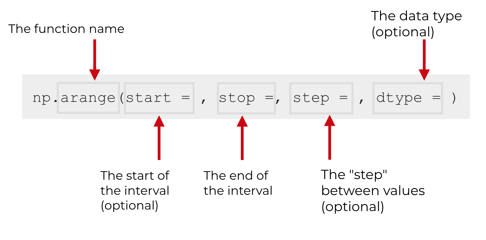
Assuming that you’ve imported NumPy into your environment as , you call the function with .

Then inside of the function, there are 4 parameters that you can modify:

Let’s take a look at each of those parameters, so you know what each one does.

(optional)
The parameter indicates the beginning value of the range.

This parameter is optional, so if you omit it, it will automatically default to 0.

(required)
The parameter indicates the end of the range. Keep in mind that like all Python indexing, this value will not be included in the resulting range. (The examples below will explain and clarify this point.) So essentially, the sequence of values will extend up to but excluding the value.

Additionally, this parameter is required, so you need to provide a value.

(optional)
The parameter specifies the spacing between values in the sequence.

This parameter is optional. If you don’t specify a value, by default the value will be 1.

(optional)
The parameter specifies the data type.

Python and NumPy have a variety of data types that can be used here.

Having said that, if you don’t specify a data type, it will be infered based on the other arguments to the function.

Numpy Arange vs Linspace vs Logspace

Let us quickly summarize between Numpy Arange, Numpy Linspace, and Numpy Logspace, so that you have a clear understanding –

1) Numpy Arange is used to create a numpy array whose elements are between the start and stop range, and we specify the step interval.

2) Numpy Linspace is used to create a numpy array whose elements are between start and stop range, and we specify how many elements we want in that range.

3) Numpy Logspace is similar to Linsace but the elements are generated based on a logarithmic scale.

• Also Read – Python Numpy Array – A Gentle Introduction to beginners
• Also Read – Tutorial – numpy.arange() , numpy.linspace() , numpy.logspace() in Python
• Also Read – Complete Numpy Random Tutorial – Rand, Randn, Randint, Normal
• Also Read – Tutorial – Numpy Shape, Numpy Reshape and Numpy Transpose in Python

Арифметические операции над массивами NumPy

Создадим два массива NumPy и продемонстрируем выгоду их использования.

Массивы будут называться и :

При сложении массивов складываются значения каждого ряда. Это сделать очень просто, достаточно написать :

Новичкам может прийтись по душе тот факт, что использование абстракций подобного рода не требует написания циклов for с вычислениями. Это отличная абстракция, которая позволяет оценить поставленную задачу на более высоком уровне.

Помимо сложения, здесь также можно выполнить следующие простые арифметические операции:

Довольно часто требуется выполнить какую-то арифметическую операцию между массивом и простым числом. Ее также можно назвать операцией между вектором и скалярной величиной. К примеру, предположим, в массиве указано расстояние в милях, и его нужно перевести в километры. Для этого нужно выполнить операцию :

Как можно увидеть в примере выше, NumPy сам понял, что умножить на указанное число нужно каждый элемент массива. Данный концепт называется трансляцией, или broadcating. Трансляция бывает весьма полезна.

The syntax of numpy power

Here, let’s just take a look at the syntax at a high level.

The syntax is really very simple, but to really “get it” you should understand exactly what the parameters are.

The parameters of np.power

In the image of the syntax above, there are two parameters:

In the official documentation for the np.power function, these are called and .

But as is often the case with the official NumPy documentation, I think those names are unintuitive. That being the case, I’m referring to and as and respectively.

(required)

The first parameter of the np.power function is .

As this implies, the argument to this parameter should be an array of numbers. These numbers will be used as the “bases” of our exponents.

Note that this is required. You must provide an input here.

Also, the item that you supply can take a variety of forms. You can supply a NumPy array, but you can also supply an array-like input. The array-like inputs that will work here are things like a Python list, a Python tuple or one of the other Python objects that have array-like properties.

Keep in mind that you can also just supply a single integer!

(required)

The second parameter is , which enables you to specify the exponents that you will apply to the bases, .

Note that just like the input, this input must be a NumPy array or an array-like object. So here you can supply a NumPy array, a Python list, a tuple, or another Python object with array-like properties. You can even provide a single integer!

Note: both arguments are positional arguments

Note that both arguments, and , are .

Positional arguments are a little confusing to beginners, but here’s a quick explanation.

How each input to np.power is used depends on where you put it inside of .

Inside of , you must put the bases first and you must put the exponents second. The position of the argument inside of determines how it is used by the function.

Note that this is in contrast to so-called “keyword arguments.” With keyword arguments, you use a particular keyword to designate an input to a function. And as long as you use the correct keywords, they can be in any order you’d like.

So essentially, if the argument is a “positional argument,” the order maters.

And because and are positional arguments, the bases must be specified first and the exponents must be specified second inside of the function.

Again, this is a little confusing, so be on the lookout for a future tutorial about positional arguments.

Python package management

Managing packages is a challenging problem, and, as a result, there are lots of
tools. For web and general purpose Python development there’s a whole
host of tools
complementary with pip. For high-performance computing (HPC),
Spack is worth considering. For most NumPy
users though, conda and
pip are the two most popular tools.

Pip & conda

The two main tools that install Python packages are and . Their
functionality partially overlaps (e.g. both can install ), however, they
can also work together. We’ll discuss the major differences between pip and
conda here — this is important to understand if you want to manage packages
effectively.

The first difference is that conda is cross-language and it can install Python,
while pip is installed for a particular Python on your system and installs other
packages to that same Python install only. This also means conda can install
non-Python libraries and tools you may need (e.g. compilers, CUDA, HDF5), while
pip can’t.

The second difference is that pip installs from the Python Packaging Index
(PyPI), while conda installs from its own channels (typically “defaults” or
“conda-forge”). PyPI is the largest collection of packages by far, however, all
popular packages are available for conda as well.

The third difference is that pip does not have a dependency resolver (this is
expected to change in the near future), while conda does. For simple cases (e.g.
you just want NumPy, SciPy, Matplotlib, Pandas, Scikit-learn, and a few other
packages) that doesn’t matter, however, for complicated cases conda can be
expected to do a better job keeping everything working well together. The flip
side of that coin is that installing with pip is typically a lot faster than
installing with conda.

The fourth difference is that conda is an integrated solution for managing
packages, dependencies and environments, while with pip you may need another
tool (there are many!) for dealing with environments or complex dependencies.

Reproducible installs

Making the installation of all the packages your analysis, library or
application depends on reproducible is important. Sounds obvious, yet most
users don’t think about doing this (at least until it’s too late).

The problem with Python packaging is that sooner or later, something will
break. It’s not often this bad,

XKCD illustration — Python environment degradation

but it does degrade over time. Hence, it’s important to be able to delete and
reconstruct the set of packages you have installed.

Best practice is to use a different environment per project you’re working on,
and record at least the names (and preferably versions) of the packages you
directly depend on in a static metadata file. Each packaging tool has its own
metadata format for this:

• Conda:

• Pip: virtual environments and

• Poetry: virtual environments and pyproject.toml

Sometimes it’s too much overhead to create and switch between new environments
for small tasks. In that case we encourage you to not install too many packages
into your base environment, and keep track of versions of packages some other
way (e.g. comments inside files, or printing after
importing it in notebooks).

Язык программирования Python

Python – это высокоуровневый, динамичный, объектно-ориентированный язык программирования. Он ориентирован на повышение производительности программиста и читаемости кода. Разработчиком кода является Гвидо ван Россум. Впервые язык увидел свет в 1991 году. При создании Python, автор вдохновлялся такими языками программирования как ABC, Haskell, Java, Lisp, Icon и Perl. Python является высокоуровневым, кроссплатформенным, но в то же время минималистичным языком. Одним из его основных преимуществ является отсутствие скобок и точек с запятой. Вместо этого Python использует отступы. Сегодня существует две основные ветви языка: Python 2.7 и Python 3.x.

Стоит отметить, что Python 3 нарушает обратную совместимость с предыдущими версиями языка. Его разработали для того, чтобы исправить ряд недостатков конструкции уже существующего языка, упростить и очистить его от ненужных деталей. Последней версией Python 2.x является 2.7.17, а Python 3.x – 3.8.5. Данный учебник написан на Python 2.x, равно как и большая часть кода. Мы обновили учебник под Python 3.8.

Для перехода программного обеспечения и самих разработчиков на Python 3.x потребуется какое-то время. Уже перешли все на Python 3. Сегодня Python поддерживается большим количеством добровольцев со всего мира. Напомню, что язык имеет открытый исходный код.

Python – это идеальный язык для тех людей, которые хотят научиться программировать.

Язык программирования Python поддерживает несколько стилей программирования. Он не принуждает разработчика придерживаться определенной парадигмы. Python поддерживает объектно-ориентированное и процедурное программирование. Существует и ограниченная поддержка функционального программирования.

Conclusion#

You now know that correlation coefficients are statistics that measure the association between variables or features of datasets. They’re very important in data science and machine learning.

You can now use Python to calculate:

• Pearson’s product-moment correlation coefficient
• Spearman’s rank correlation coefficient
• Kendall’s rank correlation coefficient

Now you can use NumPy, SciPy, and Pandas correlation functions and methods to effectively calculate these (and other) statistics, even when you work with large datasets. You also know how to visualize data, regression lines, and correlation matrices with Matplotlib plots and heatmaps.