Matplotlib tutorial: python plotting

Stateful Versus Stateless Approaches#

Alright, we need one more chunk of theory before we can get around to the shiny visualizations: the difference between the stateful (state-based, state-machine) and stateless (object-oriented, OO) interfaces.

Above, we used to import the pyplot module from matplotlib and name it .

Almost all functions from pyplot, such as , are implicitly either referring to an existing current Figure and current Axes, or creating them anew if none exist. Hidden in the matplotlib docs is this helpful snippet:

Hardcore ex-MATLAB users may choose to word this by saying something like, “ is a state-machine interface that implicitly tracks the current figure!” In English, this means that:

• The stateful interface makes its calls with and other top-level pyplot functions. There is only ever one Figure or Axes that you’re manipulating at a given time, and you don’t need to explicitly refer to it.
• Modifying the underlying objects directly is the object-oriented approach. We usually do this by calling methods of an object, which is the object that represents a plot itself.

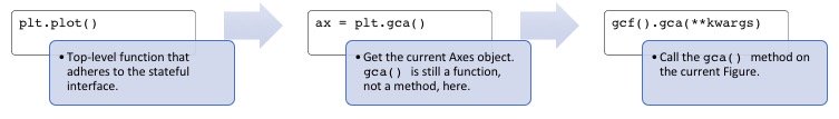
The flow of this process, at a high level, looks like this:

Tying these together, most of the functions from pyplot also exist as methods of the class.

This is easier to see by peeking under the hood. can be boiled down to five or so lines of code:

>>>

Calling is just a convenient way to get the current Axes of the current Figure and then call its method. This is what is meant by the assertion that the stateful interface always “implicitly tracks” the plot that it wants to reference.

pyplot is home to a that are really just wrappers around matplotlib’s object-oriented interface. For example, with , there are corresponding setter and getter methods within the OO approach, and . (Use of getters and setters tends to be more popular in languages such as Java but is a key feature of matplotlib’s OO approach.)

Calling gets translated into this one line: . Here’s what that is doing:

• grabs the current axis and returns it.
• is a setter method that sets the title for that Axes object. The “convenience” here is that we didn’t need to specify any Axes object explicitly with .

Диаграмма рассеяния

Это, наверное, наиболее часто используемая диаграмма при анализе данных. Она позволяет увидеть изменение переменной с течением времени или отношение между двумя (или более) переменными.

Временные ряды

В значительной части данных содержится информация о времени. К счастью, plotly + cufflinks были разработаны с расчётом на визуализацию временных рядов. Создадим DataFrame с моими статьями и посмотрим, как менялись тренды.

Здесь мы в одну строку делаем сразу несколько разных вещей:

• Автоматически получаем красиво отформатированную ось X;
• Добавляем дополнительную ось Y, так как у переменных разные диапазоны;
• Добавляем заголовки статей, которые высвечиваются при наведении курсора.

Для большей наглядности можно легко добавить текстовые аннотации:

Диаграмма рассеяния с аннотациями

А вот так можно создать точечную диаграмму с двумя переменными, окрашенными согласно третьей категориальной переменной:

Сделаем график немного более сложным, используя логарифмическую ось (настраивается через аргумент , подробнее в документации) и установив размер пузырьков в соответствии с числовой переменной:

Если захотеть (подробности в ), то можно уместить даже 4 переменные (не советую) на одном графике!

Как и раньше, мы совмещаем возможности pandas и plotly + cufflinks для получения полезных графиков:

Загляните в блокнот или документацию, чтобы увидеть больше примеров добавленной функциональности. Мы можем добавить текстовые аннотации, контрольные линии и линии тренда с помощью всего лишь одной строки кода и при этом сохраним всю интерактивность.

Intro to pyplot¶

is a collection of command style functions
that make matplotlib work like MATLAB.
Each function makes
some change to a figure: e.g., creates a figure, creates a plotting area
in a figure, plots some lines in a plotting area, decorates the plot
with labels, etc.

In various states are preserved
across function calls, so that it keeps track of things like
the current figure and plotting area, and the plotting
functions are directed to the current axes (please note that «axes» here
and in most places in the documentation refers to the axes

and not the strict mathematical term for more than one axis).

Note

the pyplot API is generally less-flexible than the object-oriented API.
Most of the function calls you see here can also be called as methods
from an object. We recommend browsing the tutorials and
examples to see how this works.

Generating visualizations with pyplot is very quick:

import matplotlib.pyplot as plt
()
('some numbers')
()

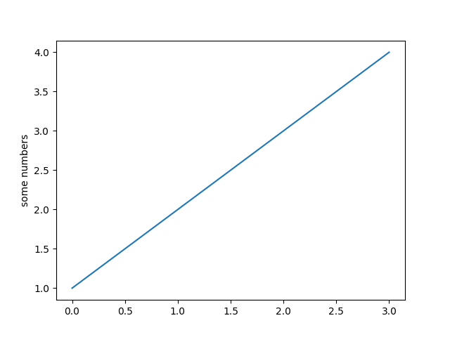
You may be wondering why the x-axis ranges from 0-3 and the y-axis
from 1-4. If you provide a single list or array to the
command, matplotlib assumes it is a
sequence of y values, and automatically generates the x values for
you. Since python ranges start with 0, the default x vector has the
same length as y but starts with 0. Hence the x data are
.

is a versatile command, and will take
an arbitrary number of arguments. For example, to plot x versus y,
you can issue the command:

(, 1, 4, 9, 16])

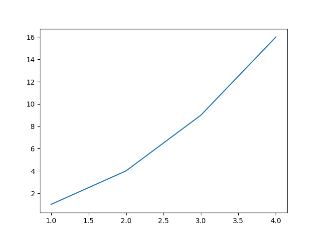
Out:

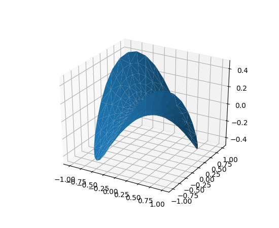
Tri-Surface plots¶

(*args, **kwargs)

Argument	Description
X, Y, Z	Data values as 1D arrays
color	Color of the surface patches
cmap	A colormap for the surface patches.
norm	An instance of Normalize to map values to colors
vmin	Minimum value to map
vmax	Maximum value to map
shade	Whether to shade the facecolors

Как начать программировать на python

The (optional) triangulation can be specified in one of two ways;
either:

plot_trisurf(triangulation, ...)

where triangulation is a
object, or:

plot_trisurf(X, Y, ...)
plot_trisurf(X, Y, triangles, ...)
plot_trisurf(X, Y, triangles=triangles, ...)

in which case a Triangulation object will be created. See
for a explanation of
these possibilities.

The remaining arguments are:

plot_trisurf(..., Z)

where Z is the array of values to contour, one per point
in the triangulation.

Other arguments are passed on to

Examples:

(Source code, png, pdf)

(Source code, png, pdf)

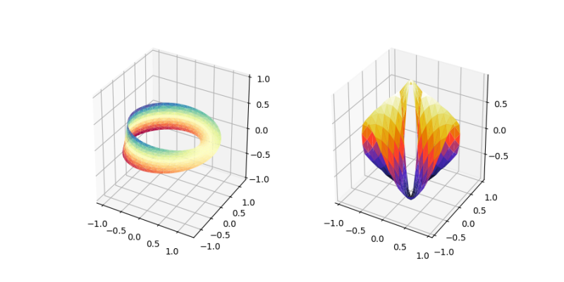
New in version 1.2.0: This plotting function was added for the v1.2.0 release.

(Source code, png, pdf)

Matplotlib

Гистограммы, созданные при помощи Matplotlib

Matplotlib это библиотека для визуализации данных, написанная на языке Python. Впервые она была выпущена еще 17 лет назад, но по-прежнему широко используется для создания графиков в сообществе Python. При создании этой библиотеки ее автор вдохновлялся MATLAB — проприетарным языком программирования, разработанным в 1980-х годах.

Поскольку Matplotlib стала первой библиотекой Python для визуализации данных, многие другие библиотеки создавались на ее основе или для использования в комбинации с ней. Некоторые из них, например, pandas и Seaborn, являются по сути врапперами Matplotlib. Они позволяют получить доступ к многочисленным методам matplotlib при помощи меньшего количества кода.

Хотя Matplotlib вполне подходит для того, чтобы разобраться в полученных данных, она не слишком хороша для быстрого и легкого создания готовых к публикации диаграмм. Как указывает Крис Моффит в своем обзоре инструментов визуализации Python, Matplotlib — «очень мощная библиотека, но при этом и сложная».

Matplotlib часто критиковали за ее дефолтный
стиль, явно воскрешающий в памяти стили
1990-х. Но в новых релизах библиотеки для
исправления этой проблемы было внесено
много изменений.

12.1.1. Описание и установка¶

Matplotlib распространяется на условиях BSD-подобной лицензии. Библиотека поддерживает двумерную (2D) и трехмерную (3D) графику, а также анимированные рисунки.

Создаваемые изображения могут быть использованы в мультимедийных приложениях, научных проектах, а также различных документах, публикациях и веб-приложениях. Исторически библиотека формировалась под влиянием математического пакета Matlab, но являлась и является независимым от него проектом. Построенная на принципах ООП, библиотека также имеет процедурный интерфейс pylab, который предоставляет аналоги команд Matlab.

Последняя стабильная версия библиотеки поддерживает Python 2.6 и выше. В курсе рассматривается matplotlib версии 2+.

Пакет поддерживает многие виды диаграмм:

• графики;

• диаграммы разброса;

• столбчатые диаграммы и гистограммы;

• круговые диаграммы;

• ствол-лист диаграммы;

• контурные графики;

• поля градиентов;

• спектральные диаграммы

• и др.

При построении возможно указать оси координат, сетку, добавить аннотации, использовать логарифмическую шкалу или полярные координаты. Созданные изображения могут быть легко сохранены, в частности, в популярные форматы (JPEG, PNG и др.).

Пример изображений приведен на Рисунке 12.1.1.

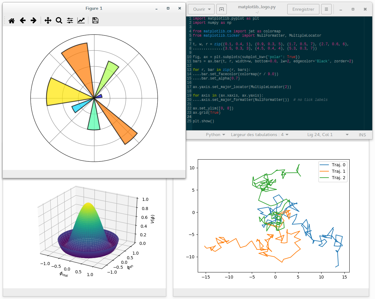
Рисунок 12.1.1 — Пример изображений, построенных с использованием matplotlib

На странице скриншотов, а также в демонстрационной галерее библиотеки приведен обширный список примеров, включающих изображения и соответствующий код.

Установка

Как и любой пакет можно установить, используя утилиту pip:

pip3 install matplotlib
pip3 install matplotlib --upgrade

Пользователям ОС на базе Linux можно воспользоваться пакетным менеджером и установить python3-matplotlib.

После установки проверьте, что библиотека имеет версию 3 и выше:

>>> import matplotlib
>>> matplotlib.__version__
'3.1.2'

Appendix B: Interactive Mode#

Behind the scenes, matplotlib also interacts with different backends. A backend is the workhorse behind actually rendering a chart. (On the popular Anaconda distribution, for instance, the default backend is Qt5Agg.) Some backends are interactive, meaning they are dynamically updated and “pop up” to the user when changed.

While interactive mode is off by default, you can check its status with or , and toggle it on and off with and , respectively:

>>>

>>>

In some code examples, you may notice the presence of at the end of a chunk of code. The main purpose of , as the name implies, is to actually “show” (open) the figure when you’re running with interactive mode turned off. In other words:

• If interactive mode is on, you don’t need , and images will automatically pop-up and be updated as you reference them.
• If interactive mode is off, you’ll need to display a figure and to update a plot.

Below, we make sure that interactive mode is off, which requires that we call after building the plot itself:

>>>

General Concepts¶

has an extensive codebase that can be daunting to many
new users. However, most of matplotlib can be understood with a fairly
simple conceptual framework and knowledge of a few important points.

Plotting requires action on a range of levels, from the most general
(e.g., ‘contour this 2-D array’) to the most specific (e.g., ‘color
this screen pixel red’). The purpose of a plotting package is to assist
you in visualizing your data as easily as possible, with all the necessary
control – that is, by using relatively high-level commands most of
the time, and still have the ability to use the low-level commands when
needed.

Therefore, everything in matplotlib is organized in a hierarchy. At the top
of the hierarchy is the matplotlib “state-machine environment” which is
provided by the module. At this level, simple
functions are used to add plot elements (lines, images, text, etc.) to
the current axes in the current figure.

Note

Pyplot’s state-machine environment behaves similarly to MATLAB and
should be most familiar to users with MATLAB experience.

The next level down in the hierarchy is the first level of the object-oriented
interface, in which pyplot is used only for a few functions such as figure
creation, and the user explicitly creates and keeps track of the figure
and axes objects. At this level, the user uses pyplot to create figures,
and through those figures, one or more axes objects can be created. These
axes objects are then used for most plotting actions.

The Matplotlib Object Hierarchy#

One important big-picture matplotlib concept is its object hierarchy.

If you’ve worked through any introductory matplotlib tutorial, you’ve probably called something like . This one-liner hides the fact that a plot is really a hierarchy of nested Python objects. A “hierarchy” here means that there is a tree-like structure of matplotlib objects underlying each plot.

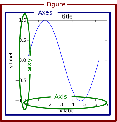
A object is the outermost container for a matplotlib graphic, which can contain multiple objects. One source of confusion is the name: an actually translates into what we think of as an individual plot or graph (rather than the plural of “axis,” as we might expect).

You can think of the object as a box-like container holding one or more (actual plots). Below the in the hierarchy are smaller objects such as tick marks, individual lines, legends, and text boxes. Almost every “element” of a chart is its own manipulable Python object, all the way down to the ticks and labels:

Here’s an illustration of this hierarchy in action. Don’t worry if you’re not completely familiar with this notation, which we’ll cover later on:

>>>

Above, we created two variables with . The first is a top-level object. The second is a “throwaway” variable that we don’t need just yet, denoted with an underscore. Using attribute notation, it is easy to traverse down the figure hierarchy and see the first tick of the y axis of the first Axes object:

>>>

Above, (a class instance) has multiple (a list, for which we take the first element). Each has a and , each of which have a collection of “major ticks,” and we grab the first one.

Matplotlib presents this as a figure anatomy, rather than an explicit hierarchy:

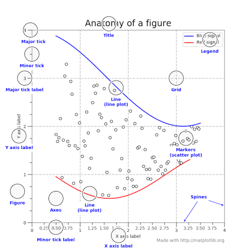
(In true matplotlib style, the figure above is created in the matplotlib docs here.)

What is interactive mode?¶

Use of an interactive backend (see )
permits–but does not by itself require or ensure–plotting
to the screen. Whether and when plotting to the screen occurs,
and whether a script or shell session continues after a plot
is drawn on the screen, depends on the functions and methods
that are called, and on a state variable that determines whether
matplotlib is in “interactive mode”. The default Boolean value is set
by the file, and may be customized like any other
configuration parameter (see ). It
may also be set via , and its
value may be queried via . Turning
interactive mode on and off in the middle of a stream of plotting
commands, whether in a script or in a shell, is rarely needed
and potentially confusing, so in the following we will assume all
plotting is done with interactive mode either on or off.

Note

Major changes related to interactivity, and in particular the
role and behavior of , were made in the
transition to matplotlib version 1.0, and bugs were fixed in
1.0.1. Here we describe the version 1.0.1 behavior for the
primary interactive backends, with the partial exception of
macosx.

Interactive mode may also be turned on via ,
and turned off via .

Note

Interactive mode works with suitable backends in ipython and in
the ordinary python shell, but it does not work in the IDLE IDE.
If the default backend does not support interactivity, an interactive
backend can be explicitly activated using any of the methods discussed in .

Interactive example

From an ordinary python prompt, or after invoking ipython with no options,
try this:

import matplotlib.pyplot as plt
plt.ion()
plt.plot()

Assuming you are running version 1.0.1 or higher, and you have
an interactive backend installed and selected by default, you should
see a plot, and your terminal prompt should also be active; you
can type additional commands such as:

plt.title("interactive test")
plt.xlabel("index")

and you will see the plot being updated after each line. This is
because you are in interactive mode and you are using pyplot
functions. Now try an alternative method of modifying the
plot. Get a reference to the instance, and
call a method of that instance:

ax = plt.gca()
ax.plot()

Nothing changed, because the Axes methods do not include an
automatic call to ;
that call is added by the pyplot functions. If you are using
methods, then when you want to update the plot on the screen,
you need to call :

plt.draw()

Now you should see the new line added to the plot.

Non-interactive example

Start a fresh session as in the previous example, but now
turn interactive mode off:

import matplotlib.pyplot as plt
plt.ioff()
plt.plot()

Nothing happened–or at least nothing has shown up on the
screen (unless you are using macosx backend, which is
anomalous). To make the plot appear, you need to do this:

plt.show()

Now you see the plot, but your terminal command line is
unresponsive; the command blocks the input
of additional commands until you manually kill the plot
window.

What good is this–being forced to use a blocking function?
Suppose you need a script that plots the contents of a file
to the screen. You want to look at that plot, and then end
the script. Without some blocking command such as show(), the
script would flash up the plot and then end immediately,
leaving nothing on the screen.

In addition, non-interactive mode delays all drawing until
show() is called; this is more efficient than redrawing
the plot each time a line in the script adds a new feature.

Prior to version 1.0, show() generally could not be called
more than once in a single script (although sometimes one
could get away with it); for version 1.0.1 and above, this
restriction is lifted, so one can write a script like this:

import numpy as np
import matplotlib.pyplot as plt
plt.ioff()
for i in range(3):
    plt.plot(np.random.rand(10))
    plt.show()

which makes three plots, one at a time.

Summary

In interactive mode, pyplot functions automatically draw
to the screen.

When plotting interactively, if using
object method calls in addition to pyplot functions, then
call whenever you want to
refresh the plot.

Use non-interactive mode in scripts in which you want to
generate one or more figures and display them before ending
or generating a new set of figures. In that case, use
to display the figure(s) and
to block execution until you have manually destroyed them.