Секционирование таблиц в oracle на практике

Example 7: Window Functions

You can use LEAD and LAG as window functions too. Window functions allow you to run the function on a certain subset of the data, called a window. For more information on window functions, read this guide on window functions.

Let’s say you wanted to find the fees paid for the previous student, and previous student was defined as someone who needed to pay the same fees or less than the current student. But it would be grouped by the required fees.

Here’s what the query would look like:

Notice a few things:

• We show both the fees_required and fees_paid
• The LAG function operates on the fees_paid column, which will show the previous record’s fees_paid value
• The PARTITION BY clause indicates how the data is partitioned or grouped for the LAG function only. In this case, it’s into partitions that have the same value for fees_required
• The ordering of data for the LAG function is by fees_required

Here are the results:

STUDENT_ID	FIRST_ NAME	LAST_ NAME	FEES_ REQUIRED	FEES_ PAID	PREV_FEES_PAID
5	Steven	Webber	100	80
6	Julie	Armstrong	100	80
9	Robert	Pickering	110	100
2	Susan	Johnson	150	150
10	Tanya	Hall	>150	>150	>150
7	Michelle	Randall	250
3	Tom	Capper	350	320
1	John	Smith	500	100
4	Mark	Holloway	500	410	100
8	Andrew	Cooper	800	400

We can see that the first row has a prev_fees_paid of null as nothing was calculated. The second row has a value of 80, because the row before it has a fees_paid of 80.

The third row has null again because there is no other record that has the same fees_required value.

The fifth row has a value of 150 because row 4 has a fees_paid value of 150.

So that’s how you can use the LAG (and LEAD) function as a window function.

You can find a full list of Oracle SQL functions here.

Lastly, if you enjoy the information and career advice I’ve been providing, sign up to my newsletter below to stay up-to-date on my articles. You’ll also receive a fantastic bonus. Thanks!

Example

The LAG function can be used in SQL Server (Transact-SQL).

Let’s look at an example. If we had an employees table that contained the following data:

employee_number	last_name	first_name	salary	dept_id
12009	Sutherland	Barbara	54000	45
34974	Yates	Fred	80000	45
34987	Erickson	Neil	42000	45
45001	Parker	Sally	57500	30
75623	Gates	Steve	65000	30

And we ran the following SQL statement:

SELECT dept_id, last_name, salary,
LAG (salary,1) OVER (ORDER BY salary) AS lower_salary
FROM employees;

It would return the following result:

dept_id	last_name	salary	lower_salary
45	Erickson	42000	NULL
45	Sutherland	54000	42000
30	Parker	57500	54000
30	Gates	65000	57500
45	Yates	80000	65000

In this example, the LAG function will sort in ascending order all of the salary values in the employees table and then return the salary that is 1 position lower in the result set since we used an offset of 1.

If we had used an offset of 2 instead, it would have returned the salary that is 2 salaries lower. If we had used an offset of 3, it would have returned the salary that is 3 lower….and so on.

Using Partitions

Now let’s look at a more complex example where we use a query partition clause to return the lower salary for each employee within their own department.

Enter the following SQL statement:

SELECT dept_id, last_name, salary,
LAG (salary,1) OVER (PARTITION BY dept_id ORDER BY salary) AS lower_salary
FROM employees;

It would return the following result:

dept_id	last_name	salary	lower_salary
30	Parker	57500	NULL
30	Gates	65000	57500
45	Erickson	42000	NULL
45	Sutherland	54000	42000
45	Yates	80000	54000

In this example, the LAG function will partition the results by dept_id and then sort by salary as indicated by . This means that the LAG function will only evaluate a salary value if the dept_id matches the current record’s dept_id. When a new dept_id is encountered, the LAG function will restart its calculations and use the appropriate dept_id partition.

As you can see, the 1st record in the result set has a value of NULL for the lower_salary because it is the first record for the partition where dept_id is 30 (sorted by salary) so there is no lower salary value. This is also true for the 3rd record where the dept_id is 45.

Развитие

Очевидно подобная микрооптимизация вовсе не стоила затраченных усилий. Можно ли качественно улучшить свойства этого окна, не изменяя исходных данных?

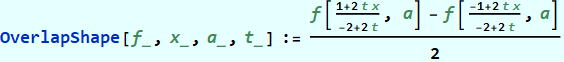
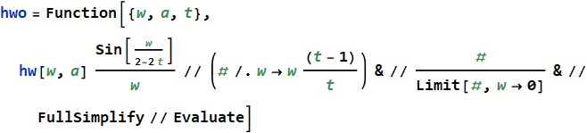
Определим вспомогательную функцию для построения перекрывающихся окон с учётом границ изменения аргумента в диапазоне от -1/2 до 1/2:

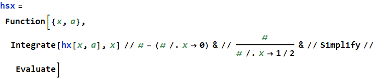
Находим первообразную, смещаем её к центру координат и масштабируем к единице:

↓

выводим её на график:

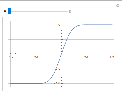
Как видим, Wolfram здесь тоже справился самостоятельно и нам не пришлось вручную задавать кусочно-непрерывное определение первообразной. Теперь вид нашего окна зависит не только от переменной a, но от степени перекрытия — и по мере его увеличения будет стремится к форме производной:

И последний штрих — найти аналитическую функцию для спектра, чтобы определить оптимальное значение параметра a.

Здесь, если мы попробуем вычислить преобразование непосредственно, как в прошлый раз — то вгоним Wolfram в глубокую задумчивость. Есть несколько способов ускорить этот процесс:

— использовать дискретное преобразование вместо аналитического — наиболее простое. Но настоящий математик не будет применять численные методы там, где можно найти чисто аналитическое решение — и мы (пока) не будем; к тому же у него есть очевидные ограничения (по разрешению и ограничению спектра);

— передавать в качестве параметра перекрытия конкретные значения и, глядя на результаты, попытаться увидеть закономерность и обобщить их. Вполне работающий вариант, но требующих дополнительных умственных и творческих усилий. Оставим его на крайний случай.

— производить вычисления непосредственно в частотном домене. Это возможно благодаря следующим свойствам преобразования Фурье:

Таким образом, имея спектр hw произвольной оконной функции, мы можем получить из него спектр hwo суммирующейся в единицу функции с перекрытием t:

↓

Теперь можно посмотреть, как меняется спектр в динамике:

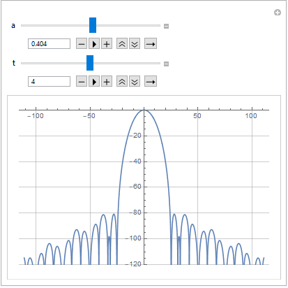
Здесь изменение параметра перекрытия уже будет влиять на спектр окна несколько по-другому:

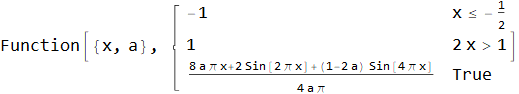
Немного поигравшись с параметрами легко заметить, что «больше — не значит лучше», и оптимальная степень перекрытия для той функции находится в районе четырёх. Конкретно, для t=4 и a=0.404 мы получаем уровень боковых лепестков, не превышающий -80 дБ. Это очень даже неплохой результат — особенно учитывая, что функция приподнятого косинуса, традиционно используемая для суммируемых в единицу окон, даёт уровень лепестков примерно в -30 дБ. Ну а выписанная явном образом наша новая оконная функция будет выглядеть так:

The ROW_NUMBER(), RANK(), and DENSE_RANK() functions

The , , and functions assign an integer to each row based on its order in its result set.

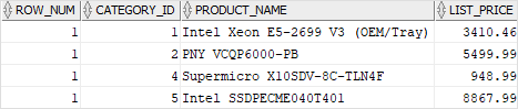
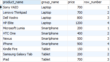
The function assigns a sequential number to each row in each partition. See the following query:

The function assigns ranking within an ordered partition. If rows have the same values, the  function assigns the same rank, with the next ranking(s) skipped.

See the following query:

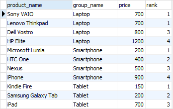
In the laptop product group, both and products have the same price, therefore, they receive the same rank 1. The next row in the group is  that receives the rank 3 because the rank 2 is skipped.

Similar to the function, the function assigns a rank to each row within an ordered partition, but the ranks have no gap. In other words, the same ranks are assigned to multiple rows and no ranks are skipped.

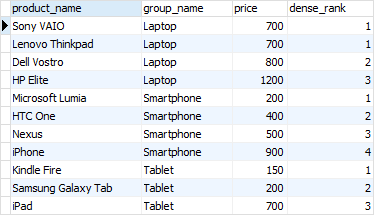
Within the laptop product group, rank 1 is assigned twice to and . The next rank is 2 assigned to .

SQL window function syntax

The syntax of the window functions is as follows:

The name of the supported window function such as , , and .

The target expression or column on which the window function operates.

clause

The clause defines window partitions to form the groups of rows specifies the orders of rows in a partition. The clause consists of three clauses: partition, order, and frame clauses.

The partition clause divides the rows into partitions to which the window function applies. It has the following syntax:

If the clause is not specified, then the whole result set is treated as a single partition.

The order clause specifies the orders of rows in a partition on which the window function operates:

A frame is the subset of the current partition. To define the frame, you use one of the following syntaxes:

where is one of the following options:

and is one of the following options:

The following picture illustrates a frame and its options:

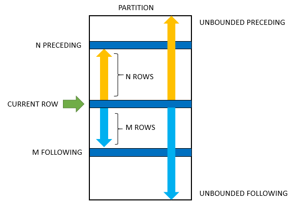
• : the frame starts at the first row of the partition.
• : the frame starts at Nth rows before the current row.
• : means the current row that is being evaluated.
• : the frame ends at the final row in the partition.
• : the frame ends at the Nh row after the current row.

The or specifies the type of relationship between the current row and frame rows.

•  : the offsets of the current row and frame rows are row numbers.
•  : the offset of the current row and frame rows are row values.

Применение

На практике нет возможности получить сигнал на бесконечном интервале, так как нет возможности узнать, какой был сигнал до включения устройства и какой он будет в будущем. Ограничение интервала анализа равносильно произведению исходного сигнала на прямоугольную оконную функцию. Таким образом, результатом оконного преобразования Фурье является не спектр исходного сигнала, а спектр произведения сигнала и оконной функции. В результате возникает эффект, называемый растеканием спектра сигнала. Опасность заключается в том, что боковые лепестки сигнала более высокой амплитуды могут маскировать присутствие других сигналов меньшей амплитуды.

Для борьбы с растеканием спектра применяют более гладкую оконную функцию, спектр которой имеет более широкий главный лепесток и низкий уровень боковых лепестков. Спектр, полученный при помощи оконного преобразования Фурье, является сверткой спектра исходного идеального сигнала и спектра оконной функции.

Искажения, вносимые применением окон, определяются размером окна и его формой. Выделяют следующие основные свойства оконных функций: ширина главного лепестка по уровню -3 дБ, ширина главного лепестка по нулевому уровню, максимальный уровень боковых лепестков, коэффициент ослабления оконной функции.

Оконное преобразование Фурье применяется в связи для синтеза частотных фильтров, например, в методе частотного мультиплексирования с множеством несущих, использующим банк (гребёнку) частотных фильтров .

LAG and LEAD

The LAG function has the ability to fetch data from a previous row, while LEAD
fetches data from a subsequent row. Both functions are very similar to each other
and you can just replace one by the other by changing the sort order.

Using the AdventureWorks data warehouse, we’ll calculate the sales amount
of the previous year.

SELECT
                              = YEAR()
    ,                 = SUM()
    ,   = LAG(SUM()) OVER (ORDER BY YEAR())
FROM .
GROUP BY YEAR()
ORDER BY ;

We can see that for each year, the data of the previous year has been fetched
in the second column:

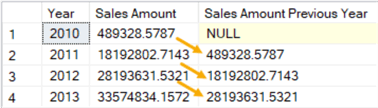
The LAG/LEAD function has also two optional parameters:

• The offset. The default is 1, but you can jump back more rows by specifying
  a bigger offset. You cannot specify a negative value.
• A default value. When there is no previous row (in the case of LAG), NULL
  is returned. You can see this in the screenshot in the first row. You can specify
  a default value to be returned instead of NULL.

If we would sort descending in the window function, LAG will fetch the next row’s
value instead of the previous one:

To show you the contrast, this is how the previous year values needed to be calculated
before LAG/LEAD were introduced:

WITH CTE_Years AS
(
    SELECT
                                  = YEAR()
        ,                 = SUM()
    FROM .
    GROUP BY YEAR()
)
, CTE_PY AS
(
    SELECT
         y1.
        ,y1.
        , = y2.
    FROM CTE_Years y1
    LEFT JOIN CTE_Years y2 ON (. + 1) = .
)
SELECT * FROM 
ORDER BY ;

As you can see, the query is a bit more elaborate since an extra step needs to
be taken: first the sales amount per year needs to be calculated, then the results
need to be joined to itself in order to fetch the data from the previous year.

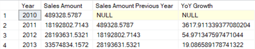
Calculating Year-over-Year growth

Using LAG, it’s easy to calculate the year-over-year growth of sales. Let’s
reuse the query from the previous example:

WITH CTE_PY AS
(
    SELECT
                                  = YEAR()
        ,                 = SUM()
        ,   = LAG(SUM())
                                            OVER (ORDER BY YEAR())
    FROM .
    GROUP BY YEAR()
)
SELECT
     
    ,
    ,
    ,                   = 100.0 * ( - )
                                        / 
FROM 
ORDER BY ;

This gives us the following result:

LEAD Function Syntax and Parameters

The syntax of the Oracle LEAD function is:

The parameters of the LEAD function are:

• expression (mandatory): An expression that is calculated and returned for the next rows. Basically, the column or value you want the function to return.
• offset (optional): The number of rows “forward” in the result set to look at. If omitted, the default is 1.
• default (optional): The value to be returned if the offset is outside the bounds of the table. By default, this is NULL.
• query_partition_clause (optional): The partitions to break the analysis into. Just like other analytic functions, it forms a kind of “group”.
• order_by_clause (mandatory): How you want to order the records to determine which row actually comes next, for this function.

Some things to know about this function:

• You can’t use nested analytics functions. So, you can’t use LEAD or any other analytics function inside the expression.
• If you want to look up the previous row instead of the next row, use the LAG function instead of LEAD.

Оконные функции: OVER(ORDER BY)

Если в определение рамки добавить предложение ORDER BY, указывающее порядок сортировки, функция начнет работать в режиме нарастания (для функции sum мы бы так и сказали — нарастающим итогом).

Для первой строки рамка будет состоять из одной этой строки; для второй — из первой и второй; для третьей — из первой, второй и третьей и так далее. Иными словами, в рамку будут входить строки с первой до текущей.

На самом деле, это можно ровно так и записать: OVER(ORDER BY… ROWS BETWEEN UNBOUNDED PRECEDING AND CURRENT ROW), но, поскольку это многословие подразумеваются по умолчанию, его обычно опускают.

Итак, рамка перестает быть статичной: ее голова движется вниз, а хвост остается на месте:

1.      2.      3.      4.      5.
+---+   +---+   +---+   +---+   +---+
| 1 |   | 1 |   | 1 |   | 1 |   | 1 |
+---+   | 2 |   | 2 |   | 2 |   | 2 |
        +---+   | 3 |   | 3 |   | 3 |
                +---+   | 4 |   | 4 |
                        +---+   | 5 |
                                +---+

PostgreSQL

Как видим, строки все так же добавляются к контексту по одной, но теперь функция average_final вызывается после каждого добавления, выдавая промежуточный итог.

Оконные функции со скользящей рамкой

Во всех примерах, которые мы посмотрели, рамка либо была статической, либо двигалась только ее голова (при использовании предложения ORDER BY). Это давало нам возможность вычислять состояние последовательно, добавляя к контексту строку за строкой.

Но рамку оконной функции можно задать и таким образом, что ее хвост тоже будет смещаться. В нашем примере это будет соответствовать понятию скользящего среднего. Например, указание OVER(ROWS BETWEEN 2 PRECEDING AND CURRENT ROW) говорит о том, что для каждой строки результата будут усредняться текущее и два предыдущих значений.

1.      2.      3.      4.      5.
+---+
|   |   +---+
|   |   |   |   +---+
| 1 |   | 1 |   | 1 |   +---+
+---+   | 2 |   | 2 |   | 2 |   +---+
        +---+   | 3 |   | 3 |   | 3 |
                +---+   | 4 |   | 4 |
                        +---+   | 5 |
                                +---+

Сможет ли вычисляться оконная функция в таком случае? Оказывается, сможет, правда неэффективно. Но, написав еще немного кода, можно улучшить ситуацию.

PostgreSQL

Посмотрим:

Вплоть до третьей строки все идет хорошо, потому что хвост фактически не двигается: мы просто добавляем к уже имеющемуся контексту очередное значение. Но, поскольку мы не умеем убирать значение из контекста, для четвертой и пятой строк все приходится пересчитывать полностью, каждый раз возвращаясь к начальному состоянию.

Итак, было бы здорово иметь не только функцию добавления очередного значения, но и функцию удаления значения из состояния. И действительно, такую функцию можно создать:

Чтобы оконная функция смогла ей воспользоваться, нужно пересоздать агрегат следующим образом:

Проверим:

Вот теперь все в порядке: для четвертой и пятой строк мы удаляем из состояния хвостовое значение и добавляем новое.

Oracle

Тут ситуация аналогична. Созданный вариант аналитической функции работает, но неэффективно:

Функция удаления значения из контекста определяется следующим образом:

Пересоздавать саму функцию не нужно. Проверим:

Introduction

Have you ever been in a situation where you needed to write a query that needed to do comparisons or access data from the subsequent rows along with the data from the current row? This article discusses different ways to write these types of queries and more specifically examines LEAD and LAG analytics functions, which were introduced with SQL Server 2012, and helps you understand how leveraging these functions can aid you in such situations.

Accessing Prior or Subsequent Rows

SQL Server 2012 introduced LAG and LEAD functions for accessing prior or subsequent rows along with the current row but before we go into the details of these functions, let me explain how you can write these queries in earlier versions of SQL Server.

Let’s first create a table and load some sample data with the script below. This table contains customer information along with when a specific plan for the customer was started, assuming when a new plan starts, the older one gets ended automatically.

DECLARE   @CustomerPlan TABLE
(
       CustomerCode VARCHAR(10),
         PlanCode   VARCHAR(10),
       StartDate  DATE
    )
INSERT INTO @CustomerPlan VALUES ('C00001', 'P00001', '1-Sep-2014')
INSERT INTO @CustomerPlan VALUES ('C00001', 'P00002', '1-Oct-2014')
INSERT INTO @CustomerPlan VALUES ('C00001', 'P00003', '10-Oct-2014')
INSERT INTO @CustomerPlan VALUES ('C00001', 'P00004', '25-Oct-2014')
INSERT INTO @CustomerPlan VALUES ('C00002', 'P00001', '1-Oct-2014')
INSERT INTO @CustomerPlan VALUES ('C00002', 'P00002', '1-Nov-2014')
 
SELECT * FROM   @CustomerPlan;

You can use Common Table Expression (CTE) along with the ROW_NUMBER ranking function to access subsequent rows in the same result set. For example, for a given customer I want to know the expiration date for the current plan based on the activation date of the next plan. Basically, when a new plan is started the previous plan is automatically ended and hence the end date for a previous plan is the start date minus one day of the next plan:

WITH   CTE as 
(
        SELECT RN = ROW_NUMBER() OVER (PARTITION BY   CustomerCode ORDER BY   StartDate ASC),   * 
        FROM @CustomerPlan
)
SELECT
        .*, 
        ISNULL(DATEADD(DAY, -1, .StartDate), '31-Dec-2099') AS EndDate
FROM   CTE 
        LEFT JOIN CTE  ON .CustomerCode   = .CustomerCode   AND  .RN   = .RN   + 1
ORDER BY .CustomerCode, .RN;

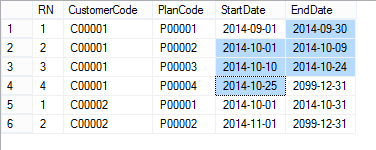
In the image above, you can see the plan P00002 of customer C00001 starts on 1st October 2014 and hence the end date for plan P00001 is the 30th September 2014 (1st October 2014 minus one day), likewise P00003 starts on 10th October and hence the end date for P00002 ends on 9th October 2014.

Examples

The examples in this topic use the allsales schema defined in Invoking Analytic Functions.

CREATE TABLE allsales(state VARCHAR(20), name VARCHAR(20), sales INT);
INSERT INTO allsales VALUES('MA', 'A', 60);
INSERT INTO allsales VALUES('NY', 'B', 20);
INSERT INTO allsales VALUES('NY', 'C', 15);
INSERT INTO allsales VALUES('MA', 'D', 20);
INSERT INTO allsales VALUES('MA', 'E', 50);
INSERT INTO allsales VALUES('NY', 'F', 40);
INSERT INTO allsales VALUES('MA', 'G', 10);
COMMIT;

Median of sales within each state
The following query uses the analytic window-partition-clause to calculate the median of sales within each state. The analytic function is computed per partition and starts over again at the beginning of the next partition.

=> SELECT state, name, sales, MEDIAN(sales)
      OVER (PARTITION BY state) AS median from allsales;

Results are grouped into partitions for MA (35) and NY (20) under the median column.

 state | name | sales | median
-------+------+-------+--------
 NY    | C    |    15 |     20
 NY    | B    |    20 |     20
 NY    | F    |    40 |     20
-------------------------------
 MA    | G    |    10 |     35
 MA    | D    |    20 |     35
 MA    | E    |    50 |     35
 MA    | A    |    60 |     35
(7 rows)

Median of sales among all states
The following query calculates the median of total sales among states. When you use with no parameters, there is one partition—the entire input:

=> SELECT state, sum(sales), median(SUM(sales))
      OVER () AS median FROM allsales GROUP BY state;
 state | sum | median
-------+-----+--------
 NY    |  75 |  107.5
 MA    | 140 |  107.5
(2 rows)

Sales larger than median (evaluation order)
Analytic functions are evaluated after all other clauses except the query’s final SQL clause. So a query that asks for all rows with sales larger than the median returns an error because the clause is applied before the analytic function and column does not yet exist:

=> SELECT name, sales,  MEDIAN(sales) OVER () AS m
   FROM allsales WHERE sales > m;
   ERROR 2624:  Column "m" does not exist

You can work around this by placing in a subquery the predicate :

=> SELECT * FROM
   (SELECT name, sales, MEDIAN(sales) OVER () AS m FROM allsales) sq
   WHERE sales > m;
 name | sales | m
------+-------+----
 F    |    40 | 20
 E    |    50 | 20
 A    |    60 | 20
(3 rows)

For more examples, see Analytic Query Examples.