Aov (average order value)

Other system performance commands

Other commands for assessing system performance include:

•  – the system reliability and load average
•  – for an overall system view
•  – vmstat reports information about runnable or blocked processes, memory, paging, block I/O, traps, and CPU.
•  – interactive process viewer
•  – helps correlate all existing resource data for processes, memory, paging, block I/O, traps, and CPU activity.
•  – interactive network traffic viewer per interface
•  – interactive network traffic viewer per process
•  – interactive I/O viewer
•  – for storage I/O statistics
•  – for network statistics
•  – for CPU statistics
•  – load average graph for terminal
•  – load average graph for X
•  – text file containing load average

Unix-style load calculation

All Unix and Unix-like systems generate a dimensionless metric of three «load average» numbers in the kernel. Users can easily query the current result from a Unix shell by running the command:

$ uptime
 14:34:03 up 10:43,  4 users,  load average: 0.06, 0.11, 0.09

The and commands show the same three load average numbers, as do a range of graphical user interface utilities. In Linux, they can also be accessed by reading the file.

An idle computer has a load number of 0 (the idle process isn’t counted). Each process using or waiting for CPU (the ready queue or run queue) increments the load number by 1. Each process that terminates decrements it by 1. Most UNIX systems count only processes in the running (on CPU) or runnable (waiting for CPU) states. However, Linux also includes processes in uninterruptible sleep states (usually waiting for disk activity), which can lead to markedly different results if many processes remain blocked in I/O due to a busy or stalled I/O system. This, for example, includes processes blocking due to an NFS server failure or too slow media (e.g., USB 1.x storage devices). Such circumstances can result in an elevated load average which does not reflect an actual increase in CPU use (but still gives an idea of how long users have to wait).

Systems calculate the load average as the of the load number. The three values of load average refer to the past one, five, and fifteen minutes of system operation.

Mathematically speaking, all three values always average all the system load since the system started up. They all decay exponentially, but they decay at different speeds: they decay exponentially by e after 1, 5, and 15 minutes respectively. Hence, the 1-minute load average consists of 63% (more precisely: 1 — 1/e) of the load from the last minute and 37% (1/e) of the average load since start up, excluding the last minute. For the 5- and 15-minute load averages, the same 63%/37% ratio is computed over 5 minutes and 15 minutes respectively. Therefore, it is not technically accurate that the 1-minute load average only includes the last 60 seconds of activity, as it includes 37% of the activity from the past, but it is correct to state that it includes mostly the last minute.

Interpretation

For single-CPU systems that are CPU bound, one can think of load average as a measure of system utilization during the respective time period. For systems with multiple CPUs, one must divide the load by the number of processors in order to get a comparable measure.

For example, one can interpret a load average of «1.73 0.60 7.98» on a single-CPU system as:

• during the last minute, the system was overloaded by 73% on average (1.73 runnable processes, so that 0.73 processes had to wait for a turn for a single CPU system on average).
• during the last 5 minutes, the CPU was idling 40% of the time on average.
• during the last 15 minutes, the system was overloaded 698% on average (7.98 runnable processes, so that 6.98 processes had to wait for a turn for a single CPU system on average).

This means that this system (CPU, disk, memory, etc.) could have handled all of the work scheduled for the last minute if it were 1.73 times as fast.

In a system with four CPUs, a load average of 3.73 would indicate that there were, on average, 3.73 processes ready to run, and each one could be scheduled into a CPU.

On modern UNIX systems, the treatment of threading with respect to load averages varies. Some systems treat threads as processes for the purposes of load average calculation: each thread waiting to run will add 1 to the load. However, other systems, especially systems implementing so-called , use different strategies such as counting the process exactly once for the purpose of load (regardless of the number of threads), or counting only threads currently exposed by the user-thread scheduler to the kernel, which may depend on the level of concurrency set on the process. Linux appears to count each thread separately as adding 1 to the load.

Quick Start

Lightweight collection of 40+ functions to retrieve detailed hardware, system and OS information.

• simple to use
• get detailed information about system, cpu, baseboard, battery, memory, disks/filesystem, network, docker, software, services and processes
• supports Linux, macOS, partial Windows, FreeBSD, OpenBSD, NetBSD and SunOS support
• no npm dependencies (for production)

Attention: this is a library. It is supposed to be used as a backend/server-side library and will definilely not work within a browser.

$ npm install systeminformation --save

All functions (except and ) are implemented as asynchronous functions. Here a small example how to use them:

constsi=require('systeminformation');si.cpu().then(data=>console.log(data)).catch(error=>console.error(error));

Callback, Promises, Awync Await

The traffic analogy

A single-core CPU is like a single lane of traffic. Imagine you are a bridge operator … sometimes your bridge is so busy there are cars lined up to cross. You want to let folks know how traffic is moving on your bridge. A decent metric would be how many cars are waiting at a particular time. If no cars are waiting, incoming drivers know they can drive across right away. If cars are backed up, drivers know they’re in for delays.

So, Bridge Operator, what numbering system are you going to use? How about:

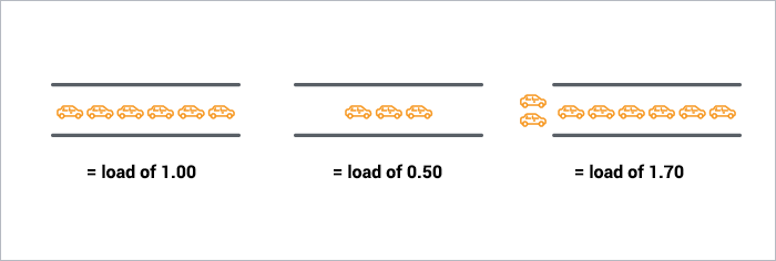
• 0.00 means there’s no traffic on the bridge at all. In fact, between 0.00 and 1.00 means there’s no backup, and an arriving car will just go right on.
• 1.00 means the bridge is exactly at capacity. All is still good, but if traffic gets a little heavier, things are going to slow down.
• over 1.00 means there’s backup. How much? Well, 2.00 means that there are two lanes worth of cars total — one lane’s worth on the bridge, and one lane’s worth waiting. 3.00 means there are three lane’s worth total — one lane’s worth on the bridge, and two lanes’ worth waiting. Etc.

This is basically what CPU load is. «Cars» are processes using a slice of CPU time («crossing the bridge») or queued up to use the CPU. Unix refers to this as the run-queue length: the sum of the number of processes that are currently running plus the number that are waiting (queued) to run.

Like the bridge operator, you’d like your cars/processes to never be waiting. So, your CPU load should ideally stay below 1.00. Also like the bridge operator, you are still ok if you get some temporary spikes above 1.00 … but when you’re consistently above 1.00, you need to worry.

Understanding Load Average in Linux

At first, this extra layer of detail seems unnecessary if you simply want to know the current state of CPU load in your system. But since the averages of three time periods are given, rather than an instant measurement, you can get a more complete idea of the change of system load over time in a single glance of three numbers

Displaying the load average is simple. On the command line, you can use a variety of commands. I simply use the “w” command:

root@virgo ~# w21:08:43 up 38 days,  4:34,  4 users,  load average: 3.11, 2.75, 2.70

The rest of the command will display who’s logged on and what they’re executing, but for our purposes this information is irrelevant so I’ve clipped it from the above display.

In an ideal system, no process should be held up by another process (or thread), but in a single processor system, this occurs when the load goes above 1.00.

The words “single processor system” are incredibly important here. Unless you’re running an ancient computer, your machine probably has multiple CPU cores. In the machine I’m on, I have 16 cores:

root@virgo ~# nproc16

In this case, a load average of 3.11 is not alarming at all. It simply means that a bit more than three processes were ready to execute and CPU cores were present to handle their execution. On this particular system, the load would have to reach 16 to be considered at “100%”.

To translate this to a percent-based system load, you could use this simple, if not obtuse, command:

cat procloadavg | cut -c 1-4 | echo «scale=2; ($(</dev/stdin)/`nproc`)*100» | bc -l

This command sequences isolates the 1-minute average via cut and echos it, divided by the number of CPU cores, through bc, a command-line calculator, to derive the percentage.

This value is by no means scientific but does provide a rough approximation of CPU load in percent.

A Minute to Learn, a Lifetime to Master

In the previous section I put the “100%” example of a load of 16.0 on a 16 CPU core system in quotes because the calculation of load in Linux is a bit more nebulous than Windows. The system administrator must keep in mind that:

• Load is expressed in waiting processes and threads
• It is not an instantaneous value, rather an average, and
• It’s interpretation must include the number of CPU cores, and
• May over-inflate I/O waits like disk reads

Because of this, getting a handle of CPU load on a Linux system is not entirely an empirical matter. Even if it were, CPU load alone is not an adequate measurement of overall system resource utilization. As such, an experienced Linux administrator will consider CPU load in concert with other values such as I/O wait and the percentage of kernel versus system time.

I/O Wait

I/O wait is most easily seen via the “top” command:

In the screenshot above I have highlighted the I/O wait value. This is a percentage of time that the CPU was waiting on input or output commands to complete. This is usually indicative of high disk activity. While a high wait percentage alone may not significantly degrade CPU-bound tasks, it will reduce I/O performance for other tasks and will make the system feel sluggish.

High I/O wait without any obvious cause might indicate a problem with a disk. Use the “dmesg” command to see if any errors have occurred.

Kernel vs. System Time

The above highlighted values represent the user and kernel (system) time. This is a breakdown of the overall consumption of CPU time by users (i.e. applications, etc.) and the kernel (i.e. interaction with system devices). Higher user time will indicate more CPU usage by programs where higher kernel time will indicate more system-level processing.

Troubleshooting

The factual accuracy of this article or section is disputed.

Some applications, like ntop, do not respond well to automatic frequency scaling. In the case of ntop it can result in segmentation faults and lots of lost information as even the on-demand governor cannot change the frequency quickly enough when a lot of packets suddenly arrive at the monitored network interface that cannot be handled by the current processor speed.

Some CPU’s may suffer from poor performance with the default settings of the on-demand governor (e.g. flash videos not playing smoothly or stuttering window animations). Instead of completely disabling frequency scaling to resolve these issues, the aggressiveness of frequency scaling can be increased by lowering the up_threshold sysctl variable for each CPU. See how to change the on-demand governor’s threshold.

Sometimes the on-demand governor may not throttle to the maximum frequency but one step below. This can be solved by setting max_freq value slightly higher than the real maximum. For example, if frequency range of the CPU is from 2.00 GHz to 3.00 GHz, setting max_freq to 3.01 GHz can be a good idea.

Some combinations of ALSA drivers and sound chips may cause audio skipping as the governor changes between frequencies, switching back to a non-changing governor seems to stop the audio skipping.

BIOS frequency limitation

Some CPU/BIOS configurations may have difficulties to scale to the maximum frequency or scale to higher frequencies at all. This is most likely caused by BIOS events telling the OS to limit the frequency resulting in set to a lower value.

Either you just made a specific Setting in the BIOS Setup Utility, (Frequency, Thermal Management, etc.) you can blame a buggy/outdated BIOS or the BIOS might have a serious reason for throttling the CPU on it’s own.

Reasons like that can be (assuming your machine’s a notebook) that the battery is removed (or near death) so you’re on AC-power only. In this case a weak AC-source might not supply enough electricity to fulfill extreme peak demands by the overall system and as there is no battery to assist this could lead to data loss, data corruption or in worst case even hardware damage!

If you checked there’s not just an odd BIOS setting and you know what you’re doing you can make the Kernel ignore these BIOS-limitations.

Warning: Make sure you read and understood the section above. CPU frequency limitation is a safety feature of your BIOS and you should not need to work around it.

A special parameter has to be passed to the processor module.

For trying this temporarily change the value in from to .

For setting it permanently describes alternatives. For example, you can add to your kernel boot line, or create

/etc/modprobe.d/ignore_ppc.conf

# If the frequency of your machine gets wrongly limited by BIOS, this should help
options processor ignore_ppc=1

What about Multi-processors? My load says 3.00, but things are running fine!

Got a quad-processor system? It’s still healthy with a load of 3.00.

On multi-processor system, the load is relative to the number of processor cores available. The «100% utilization» mark is 1.00 on a single-core system, 2.00, on a dual-core, 4.00 on a quad-core, etc.

If we go back to the bridge analogy, the «1.00» really means «one lane’s worth of traffic». On a one-lane bridge, that means it’s filled up. On a two-late bridge, a load of 1.00 means its at 50% capacity — only one lane is full, so there’s another whole lane that can be filled.

Same with CPUs: a load of 1.00 is 100% CPU utilization on single-core box. On a dual-core box, a load of 2.00 is 100% CPU utilization.

Bringing It Home

Let’s take a look at the load averages output from :

~ $ uptime23:05 up 14 days, 6:08, 7 users, load averages: 0.65 0.42 0.36

This is on a dual-core CPU, so we’ve got lots of headroom. I won’t even think about it until load gets and stays above 1.7 or so.

Now, what about those three numbers? 0.65 is the average over the last minute, 0.42 is the average over the last five minutes, and 0.36 is the average over the last 15 minutes. Which brings us to the question:

Which average should I be observing? One, five, or 15 minute?

For the numbers we’ve talked about (1.00 = fix it now, etc), you should be looking at the five or 15-minute averages. Frankly, if your box spikes above 1.0 on the one-minute average, you’re still fine. It’s when the 15-minute average goes north of 1.0 and stays there that you need to snap to. (obviously, as we’ve learned, adjust these numbers to the number of processor cores your system has).

So # of cores is important to interpreting load averages … how do I know how many cores my system has?

to get info on each processor in your system. Note: not available on OSX, Google for alternatives. To get just a count, run it through and word count: